Chapter 1 Estimating Fish Abundance from the Behavior of Fishing Fleets
1.1 Introduction
Successful fisheries management rests in part on the ability to provide accurate and timely assessments of the status (generally in the form of biomass levels and/or fishing mortality rates relative to some reference point) of fish stocks. Fisheries science has developed an expansive and often effective toolbox for providing this knowledge, but the data-intensive nature of many of these tools has prevented their use in all but the most knowledge and resource rich parts of the world. In recent years, this problem has led to an rapid expansion of “data-limited assessments” (DLAs), that seek to provide stock status estimates using fewer data (but more assumptions) for fisheries that do not have for formal stock assessments in place (such as those encompassed by the RAM Legacy Stock Assessment Database, Ricard et al. 2012). While length-based DLAs are commonly used at the more local level (e.g. Hordyk et al. 2014; Rudd and Thorson 2017), at larger spatial scales catch-based methods, that try to explain stock status as a function of trends in the amount of fish caught from a population, have become the standard method (e.g. Costello et al. 2012, 2016; Rosenberg et al. 2017).
This prevalence of catch-based methods is based largely out of necessity rather than performance; catch statistics, such as those provided by the Food and Agriculture Organization of the United Nations (FAO; FAO (2018)), have been to date the only globally available source of fishery statistics. While these catch-based methods have been shown to be effective in some circumstances (Anderson et al. 2017; Rosenberg et al. 2017), catch statistics alone can be misleading in understanding stock status (Pauly et al. 2013). The need for expanded tools to rapidly understand and manage data-limited fisheries is increasingly critical as populations grow and the climate changes. Global Fishing Watch, presented by Kroodsma et al. (2018), presents a new global database of fishing effort, updated in near real time. Can these new data be used to improve our ability to understand the status of fisheries around the world?
Why might we think that data on the dynamics of fishing effort might be useful for fisheries stock assessment? Regardless of their scale, from large industrial operations to small artisanal activity, fisheries share a common underlying incentive structure: fishermen desire some utility derived from capturing fish (e.g. some combination of food, income, and cultural activity) and tune their fishing activities in order to try and maximize that utility, subject to the constraints of the world. As time goes on, these fishing actions affect fish stocks, for example through reductions in abundance or mean length, causing the behavior of the fishermen to be updated. In short then, fishing and fish are part of a dynamic system, in which the behavior of each affects the behavior the other.
These dynamic links between fishing fleets and fish populations are a critical part of fisheries management. Gordon (1954) predicted that in the absence of property rights or access restrictions, these bio-economic dynamics would result in the fishery reaching an open-access equilibrium at which net profits in the fishery are driven to zero, often resulting in biological overfishing of the stock. This thinking was central to the bleak predictions of the “tragedy of the commons” (Hardin 1968). While Ostrom (1990) demonstrated that the evolution of natural resource systems such as fisheries are driven by a more complete and complex set of drivers than pure profitability, the critical link between the dynamics of fish populations and fishing communities remains in the form of social-ecological systems (Ostrom 2009).
Understanding the dynamics of these social-ecological systems is critical to effective fisheries management. Bio-economic theory and empirical evidence helps us design and implement policies that best achieve societal objectives, by allowing us to model what the potential impacts of policy choices may be. This process has underpinned the recent expansion in the use of rights-based fisheries management (Grafton 1996; Cancino et al. 2007; Deacon and Costello 2007; e.g. Costello and Polasky 2008; Kaffine and Costello 2008; Wilen et al. 2012; Grainger and Costello 2016; Costello et al. 2016; Squires et al. 2016), and increasingly is used in the management-strategy-evaluation process (MSE, Butterworth 2007; Punt et al. 2016). Nielsen et al. (2017) provides a thorough review of models currently utilizing bio-economic modeling to model and guide the policy implementation process.
These works demonstrate a rich history of thinking about how fishing fleets respond to incentives and population dynamics. However, the vast majority of the literature in this field is focused on predicting fishing effort as a function of fish populations; relatively little research has reversed this question and asked, what do the dynamics of fishing effort suggest about the state of fish populations? If fisheries are indeed a coupled bio-economic system, then just as we believe the dynamics of fishing effort should be predictable from fish abundance, fish abundance should be predictable from fishing effort (Sugihara et al. 2012). Prince and Hilborn (1998) and Hilborn and Kennedy (1992) both provide empirical evidence for this relationship, by demonstrating how the economics of fishing interact with spatio-temporal population dynamics. Their results show that as a fishery nears equilibrium, the spatial distribution of effort should reflect the spatial distribution of abundance. However, while these results demonstrate a predictable link between effort and abundance, we know of few examples in the stock assessment literature of attempting to use effort alone to estimate abundance. This is likely partly due simply to the history of stock assessment as a biological science (Smith 1994), and partly due to data realities. Historically, most fisheries with say accurate and complete records of fishing effort would also have records of more directly useful (from the perspective of traditional stock assessment) indices such as catches and catch-per-unit-effort. In these cases the catch data, combined with catch-per-unit-effort (CPUE) data, can in theory provide a clearer signal of the state of a fish stock (with the catch data providing information on the scale of abundance and CPUE data on trends) than the effort data.
While effort dynamics have not been historically used to understand fish populations, it is reasonable to believe that given sufficient data, it should be possible to infer something about the state of a fish population as a function of the behavior of fishing fleets. This idea is in many ways analogous to earlier research linking the behavior of sea birds and the location of their prey (Furness and Camphuysen 1997). While this general link between effort and abundance is grounded in sound theory, the actual form of link between fishing effort and fish abundance is far from clear. High levels of fishing effort could reflect high abundance of fish in the earlier years of a fishing ground, or could reflect a relatively depleted but easily accessible region. In addition, the rate at which fishing effort responds to abundance may depend critically on the availability of alternative fishing or employment opportunities. We hypothesize that all else equal, fishermen would like to maximize their utility from fishing, but the varied and complex nature of these individual utility functions, combined with the shifting and uncertain nature of the natural world, make the structure of the link between fishing behavior and fish abundance a complicated question.
Empirical evidence and theory suggest that a) there is a link between effort and abundance but that b) the dynamics of those linkages can be complicated. This project tests the ability of different models to untangle these dynamics and use effort data from Global Fishing Watch to make accurate predictions of both the spatial distributions and relative trends of fish abundance. We do this by pairing these effort data with fishery-independent research surveys compiled by the FishData (as described in Thorson et al. 2015) package in R (R Core Team 2018) to ask, can GFW derived effort data be used to predict the abundance of fish?
We break this assessment into a series of phases.
We assess the relationships between total effort and biomass indices in order to see if, simply put, more more fishing is associated with more or less fish
We assess whether total effort can be paired with regional catch data to create an index of catch-per-unit-effort which in turn provides a reasonable index of fish abundance over time
We consider the ability of a series of structural economic models, based on bio-economic theory, to predict fish abundance as a function of fishing behavior
We compare the predictive performance of the structural models to a suite of machine-learning models that utilize the same GFW data, and available covariates if desired, to predict fish abundance
Lastly, we consider the predictive value of GFW derived information relative to other globally available indices (e.g. sea surface temperature and chlorophyll)
1.2 Methods
1.2.1 Picking Models for Prediction
Assuming that methods such as the fishery independent research surveys used in this study represent our best estimates of biomass of fish in an area (i.e. that metrics such as effort do not somehow provide better estimates of status than the surveys, which seems a safe assumption), the ability of effort to predict abundance is useful only if we have reasonable belief that it will work in places that have effort data but do not have research surveys. For example, we could envision using this proposed effort-based model in locations that are covered by Global Fishing Watch but not by research surveys (which would represent most of the globe), or in between survey years for non-annual research surveys (e.g. those in the Aleutian Islands or the Gulf of Alaska).
We need then some method for judging which candidate models are likely to be the best at out-of-sample prediction. We did this by following the framework laid out in Kuhn and Johnson (2013). We first took our merged database of fishing effort and fish abundance and created a series of training and testing splits. These training splits were then used for all model fitting and judging. The testing splits were held aside until model selection based on the training data was complete, at which time we tested the ability of the tuned models to predict the density of fishes reported in the testing data. This specific step is critical to selecting the model with highest chance of providing good out-of-sample prediction. Even if the testing splits are not used in the fitting directly, repeatedly fitting the models to the training data and inspecting the performance against the testing data introduces an element of bias where the selected model may be the one that happens to do best for that specific test-training split, and as such is not truly independently tuned for out-of-sample prediction.
We created a large number of candidate test and training splits, in order to compare the sensitivity of the model selection process during the training phase to the specific splitting.
random- The data were split using stratified random sampling from within the survey regions (to ensure that all regions were proportionally covered)
california- We split the data into a training set of data off of the coasts of the states of Washington and Oregon, and used data off of California for the testing split. This split helps us evaluate whether a model fit to one region can be extrapolated to another region, albeit a roughly similar one in some areas.
future- We split the data into a training set composed of data from 2012:2013, and held out all data from the years 2014:2017 for the testing split. This gives an estimate of the model performance in time periods not covered by the training data.
For the sake of clearer results, we only present our diagnostics of the model fitting to the training data using the random split, but we return to the california, and future splits when we confront the selected models to the testing splits.
1.3 Methods
The broad steps of this project are
- Create a merged database of fishing effort and fish abundance, along with relevant covariates
- Fit a series of candidate models across a variety of spatial resolutions and data splits
- Evaluate the overall fit of each of the models and select those with highest change of performing well out of sample
- Examine the value of information of effort data relative to environmental data (for predicting abundance)
- Assess the predictive performance, both in space and time, of selected models
1.3.1 Data
GFW provides data on the amount and location of fishing effort, along with available observed or estimated covariates such as vessel size, distance from shore/port, and engine power. Estimates of fish abundance (measured as density or biomass) in space and time were obtained from their relevant surveys through the FishData package. The following two data sections provide summaries of the data as well as descriptions of relevant data processing steps taken.
1.3.1.1 Trawl Survey Data
FishData provides access to numerous fishery independent research surveys throughout the world. We use the bottom trawl surveys conducted along the west coast of North America by the National Marine Fisheries Service (Fig.1.1)
- Eastern Bering Sea Bottom Trawl Survey (ebsbts)
- Aleutian Islands Bottom Trawl Survey (aibts)
- Gulf of Alaska Bottom Trawl Survey (goabts)
- West Coast Groundfish Bottom Trawl Survey (wcgbts)
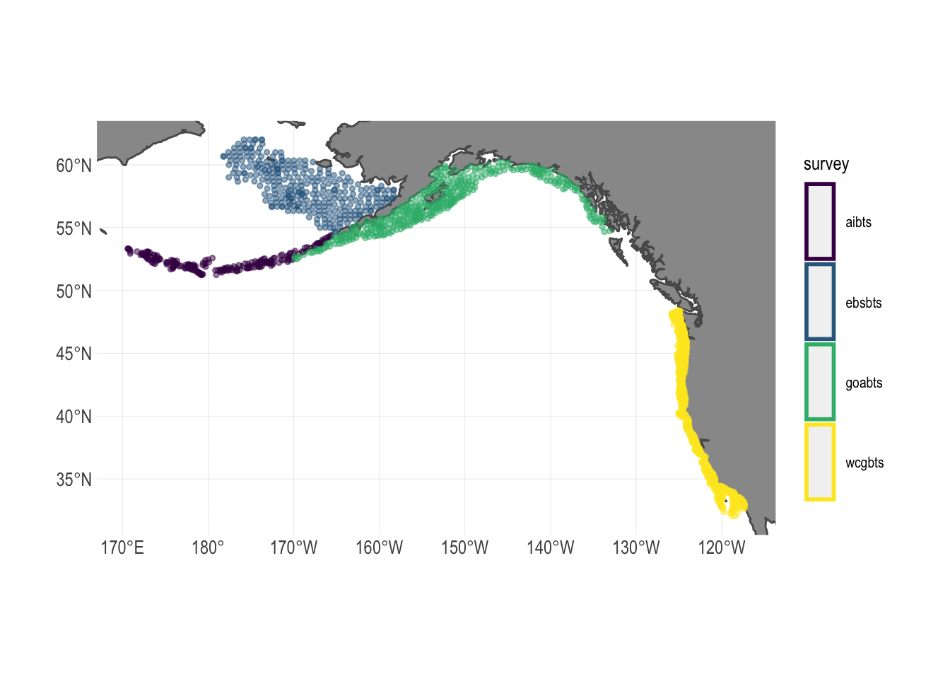
Figure 1.1: Spatial coverage of fishery independent research surveys used in this study. Names represent abbreviated survey regions
Each of the surveys contains data on a wide variety of different species, including highly abundant fished species such as Arrowtooth Flounder (Atheresthes stomias) and Alaska Pollock (Gadus chalcogrammus), as well as unfished species such as miscellaneous sea anemones (order Actiniaria). The selected surveys utilize bottom trawl gear, and as such primarily contain bottom-associated species (Fig.1.2). Surveys are conducted in summer months (July-August for the Alaska surveys and May-October for the West Coast Bottom Trawl Survey).
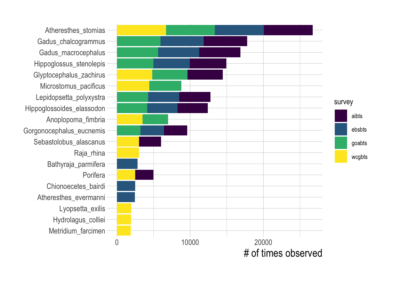
Figure 1.2: Number of positive encounters for the top-10 most observed species in each research survey
Survey data are provided by FishData in their “raw” form (biomass by species per unit of survey effort at a given sampling event). The data therefore require standardization to account for differences in vessel characteristics, spatio-temporal correlation structures, and the presence of zeros in the haul data. This standardization was performed using the VAST package (Thorson et al. 2016), which implements a spatial delta-generalized linear mixed model to provide a standardized spatio-temporal index of abundance for each species in the data. While versions of VAST allow for accounting of both within and across species correlations, we chose to run the standardization process separately for each species for the sake of convergence time (tests of this choice on smaller subsets of the data indicate the differences between the two approaches are not substantial).
The result of VAST is a network of “knots” that define polygons of equal density for each species, where the density of each species is measured in units of metric tons/km2 (Fig.1.3).
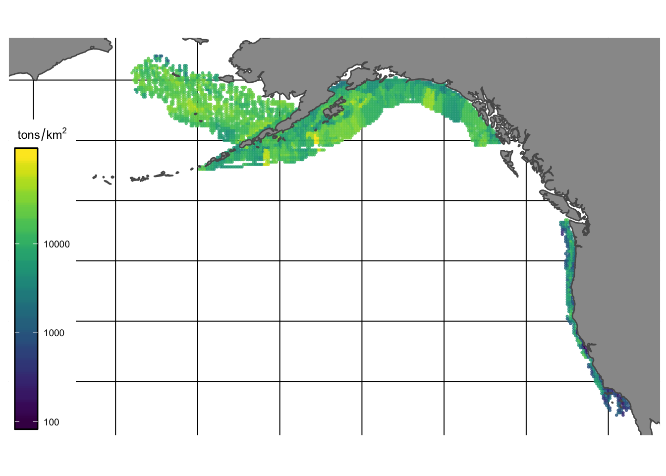
Figure 1.3: VAST estimates of density (tons/km2) of species observed in bottom trawl surveys for the Alaska region - NOTE seems like problem in reported units of trawl survey of AIBTS
Surveyed species vary substantially in their economic importance. We mark species encountered in the surveys as “fished” if their name, or a synonym for their name identified through the taxize package, was found within the global catch records of the Food and Agriculture Organization of the United Nations (FAO 2018). For each species, we also obtained price estimates using the data provided by Melnychuk et al. (2016). Together, these data provide estimated density for fished species encountered by the US west coast bottom trawl survey program over space and time, along with the associated value of these species. This allows us to examine both the density of species, and the “revenue density” available for fishing in different locations (Fig.1.4).
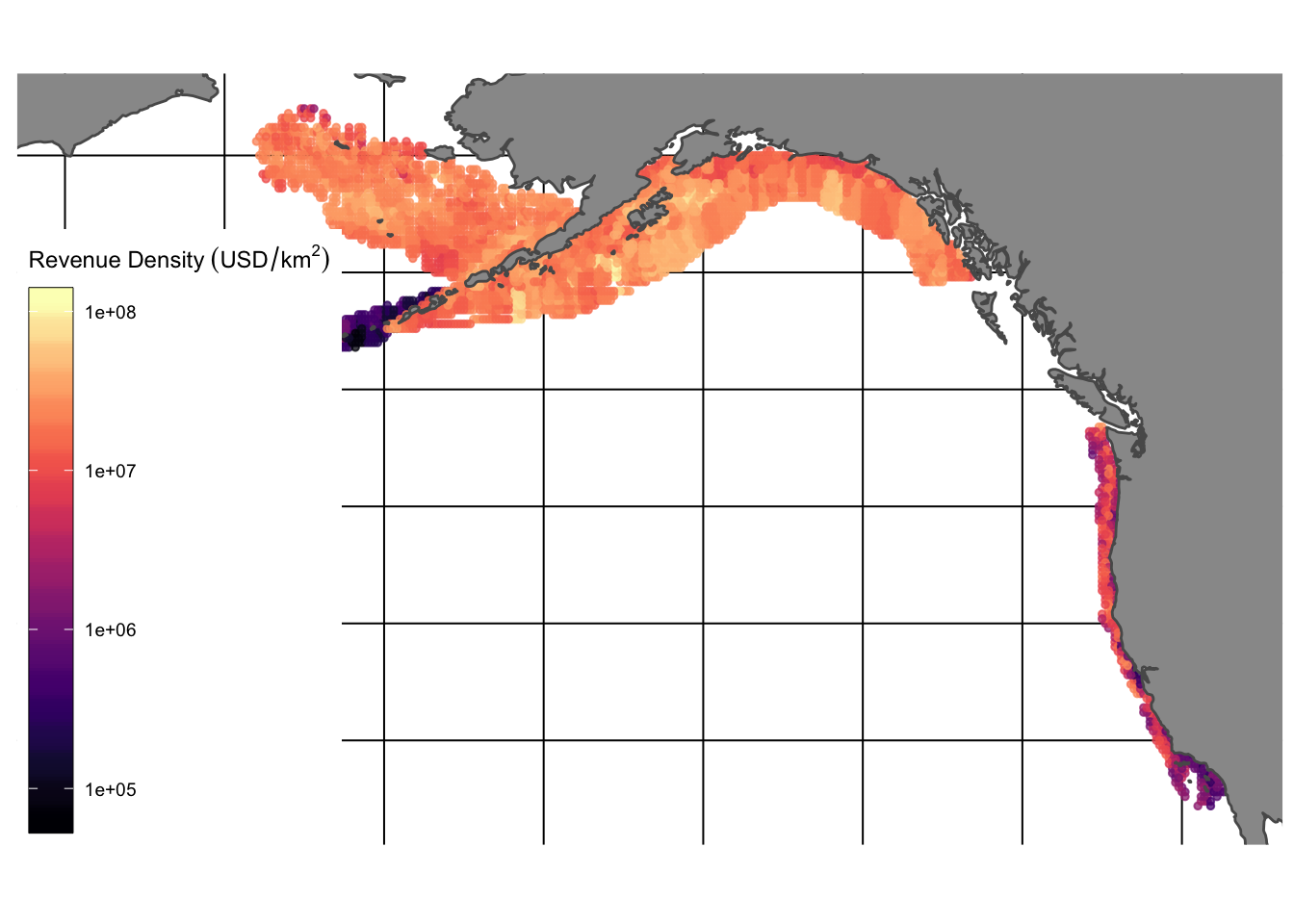
Figure 1.4: Estimated fishing revenue density ($/km^2)
1.3.1.2 Fishing Effort Data
Fishing effort data were obtained using the bigrquery package in R from Global Fishing Watch. Data were aggregated to the resolution of year and nearest 0.2 degree latitude and longitude, and for each vessel at this a given location we calculated the total fishing hours spent there, average distance from shore, average distance from port, and whether that location is inside an MPA (and if so whether the MPA was no-take or restricted-use). We also collected relevant data for that vessel such as its engine power, length, tonnage, and vessel type (trawler, purse-seine, fixed-gear, etc). Together, these data provide fishing effort-related data covering the regions surveyed in our fishery-independent data (1.5).
Global Fishing Watch uses a neural-net to classify observed behavior as fishing or not fishing (Kroodsma et al. 2018) From there, we filtered out the classified fishing behavior to entries that were more than 500m offshore, were moving faster than 0.01 knots and slower than 20 knots, to remove likely erroneous fishing entries.
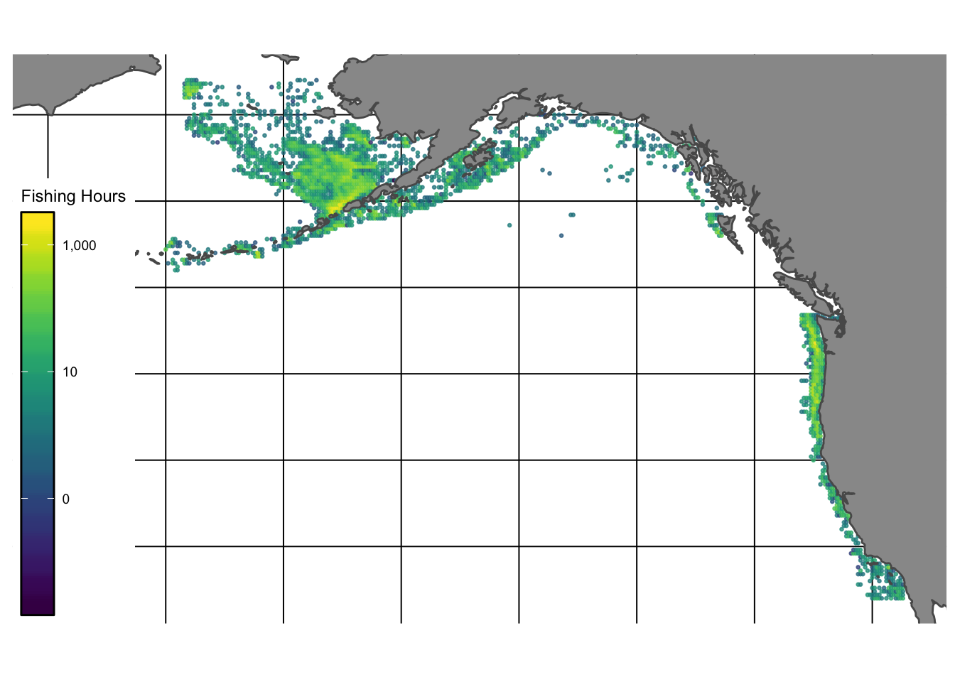
Figure 1.5: Total hours of fishing activity reported by Global Fishing Watch in the Eastern Bering Sea, Aluetian Islands, and Gulf of Alaska regions
1.3.1.3 Environmental Covariates
We augmented the effort and abundance data with globally accessible environmental covariates of
- Chlorophyll
- Sea surface temperature
- Bathymetry
All data were obtained from NOAA ERDDAP portal, and aggregated as needed to match the resolution of the GFW data (annual and 0.2 degree lat/long resolution). Other environmental data were explored (e.g. wave and wind), but did not have sufficient near-shore coverage for inclusion in the model.
1.3.1.4 Creating Merged Database
Having pulled together data on fish abundance, fishing effort, and environmental covariates, we then merged these data together into a comprehensive database. Effort data and environmental data were first merged together by matching year and location (as measured by latitude and longitude). The combined data were then clipped to only include observations that fall within the boundaries of the polygons defined by each trawl survey (Fig.1.1). From there, we snapped each effort-environment observation to the nearest (in terms of latitude and longitude distance) knot of fish abundance as defined by the VAST standardization process. Since the survey data are generally at a courser resolution than the effort data, this means that multiple effort observations are often associated with any one knot at any one time.
We then performed a series of filtering steps on this merged database. Since all surveys are geared towards bottom dwelling species, only bottom-associated gears are included from the effort data. In this case that means vessels identified by Global Fishing Watch as trawlers, pots and traps, and set gears (bottom longline and gillnet). We also only included species that were observed 10 or more times during each year of the survey to improve model convergence. To account for potential seasonal shifts in abundance, we also filtered the data down to months in which the relevant research trawl surveys were conducted.
This final merged database provides effort data at the resolution of effort per 0.2 degree2 per year, and abundance at the resolution of “knot” per year, where the exact area of each knot varies. Each observation of effort is then paired to the spatially nearest knot of abundance estimates This leaves open a question of at what resolution do we wish to fit the models? At the temporal scale, we can only fit to annual data, since that is the temporal resolution of the abundance estimates. On the spatial scale though, at the finest resolution we can use a 0.2 degree2 spatial resolution, or we could aggregate all the data up to a total abundance estimate each year. The challenge here is a trade-off between decreasing noise but also decreasing degrees of freedom. Since we only have at most six years of data (and some regions less), aggregating all data together to the annual scale would leave us with only six datapoints. While we explore some visual assessments of this idea, six datapoints do not leave us much room for model fitting. At the other end of the scale, using the finest resolution data gives us a very large sample size, but also means we are trying to predict abundances at a very fine spatial scale. So, even if the goal of the model is to predict time trends, we still fit the model using finer resolution spatial data, and then aggregate predictions together if we wish to examine time trends.
1.3.2 Candidate Predictive Models
We evaluated three classes of candidate models for linking fishing effort to fish abundance:
- Linear models
- These simply link abundance to effort through linear models.
- Structural economic models
- These assume a non-linear functional form to the allocation of fishing effort, the parameters of which are tuned to available data conditional on these structural assumptions.
- Machine learning models
- These models make no explicit structural assumptions, but rather find the combination of predictor variables that maximize the out-of-sample predictive power of the model
The choice of evaluating both structural and machine learning models is important to discuss for a moment. Substantial amounts of empirical evidence and bio-economic theory exists hypothesizing how fishing effort and fish abundance might be related, from relatively classical ideal-free distributions (e.g. Miller and Deacon 2016) to more complex agent-based approaches (e.g. Vermard et al. 2008). These structural models have the advantage of interpretability, but leave us open to errors in model specification. In contrast, machine learning models lose interpretability but are less sensitive to specification errors. While different in their mechanics, all the candidate machine learning models are black-box models whose sole objective is to maximize the predictive power of the model (as defined by the user). The user specifies some model options, but the model decides which data are important and how those data relate to each other. This allows these algorithms to fit highly non-linear models (if the data demand it), without the need to specify an exact statistical or structural form for how variables such as costs, safety, and fish abundance interact to affect fishing behavior.
As a result, machine learning models can serve as an effective benchmark for the best possible ability of GFW data to predict fish abundance. The disadvantage is that, while new techniques are emerging for interpreting machine learning model fits, they are inherently black boxes and as such do not permit us to really interpret the meaning of specific coefficients. The lack of a structural theory behind the model may also hamper the ability of these models to predict radically out of sample data (e.g. a machine learning model trained in Alaska may perform terribly in Africa). By fitting both structural and machine learning models, we can compare the machine learning and structural approach and see how much the interpretability of the structural model “costs” us in terms of predictive power, relative to the benchmark of the machine learning model.
1.3.3 Linear Models
We include the linear models purely for data exploration (though if they happen to work well they could be used). The linear models include simple linear regressions between metrics of effort and metrics of abundance (e.g. total engine hours against total biomass). We also consider CPUE trends as a class of linear model (since it is just a linear transformation of the effort data), where we now ask is, is a Global Fishing Watch index of CPUE proportional to abundance? We tested one slightly more involved linear model, of the form
\[(E_{y,k}) \sim Gamma(cost_{y,k} + \hat{B_{y,k}}, shape, scale)\]
\[ \hat{B_{y,k}} \sim normal(\bar{B_{survey}}, \sigma_{survey})\]
Where \(E_{y,k}\) is the observed total effort in year y for knot (location) k, cost is our linear cost function, and \(\hat{B}\) is a estimate of the effect for each knot, drawn from a distribution within each survey with mean \(\bar{B_{survey}}\). In order for \(\hat{B}\) to in fact be representative of fish biomass at a location, the assumption is that all of the other attributes that affect the decision of how much effort to allocate at a given site are captured by the estimated cost coefficient, which we assume is a linear function of the distance of a knot k from port, the distance from shore, the depth at that location, and the mean vessel size used at that observation. We used a Bayesian hierarchical model implemented through the rstanarm package to estimate this linear model. We then extracted the estimated \(\hat{B}\) coefficients, and compared them to the fish biomass estimated at that location by the relevant fishery independent survey.
1.3.4 Structural Models
Our structural models are constructed in the same manner as Miller and Deacon (2016). The key of this model is the assumption that for a given spatio-temporal resolution, fishermen distribute themselves such that marginal profits are equal in space.
Following Miller and Deacon (2016), we consider marginal profits \(\Pi\) per unit effort as being
\[\Pi_{y,k} = pqB_{y,k}e^{-qE_{y,k}} - c_{y,k}\]
where for year y at knot k, p is price (drawn from Melnychuk et al. 2016), B is our index of abundance (from the trawl surveys and VAST), q is catchability, E is effort (supplied by Global Fishing Watch), and c are variable costs).This leaves q and c as the unknowns in this equation.
Miller and Deacon (2016) were primarily interested in estimating quota price aspects of c, taking as data p, CPUE, E, and other components of c (fuel, labor, ice, etc.). We are instead interested in estimating CPUE as a function of other variable, and so we can rearrange this equation to construct a model of the form
\[log(B_{y,k}) \sim normal(\frac{\Pi_{y,k} + c_{y,k}}{pqe^{-qE_{y,k}}}, \sigma_B)\]
Similar to Miller and Deacon (2016) we assume for now that \(\Pi_{y,k}\) is zero, though this is clearly not accurate given that many of the fisheries encompased by the data are highly regulated and in some cases rationalized (however, changing \(\Pi_{y,k}\) to positive values had little effect on the fit of the model during trial runs). That leaves q and c as unknown parameters. While we do not have the high resolution logbook data available to Miller and Deacon (2016), we could certainly obtain data on fuel and labor prices for this model. However, at this time, we simply assume that \(c_{y,k}\) is a linear function of the distance of a knot k from port, the distance from shore, the depth at that location, and the mean vessel size used at that observation. We fit this model, estimating q and the cost coefficients and \(\sigma_B\) using maximum likelihood with the Laplace approximation implemented with Template Model Builder (TMB, Kristensen et al. (2016)) in R.
This form of the model assumes the goal is to estimate B directly. Use of this model for prediction in new locations would require assuming that the fitted q and cost values are applicable to a new location. An alternative approach is to estimate a vector of latent variables \(\hat{B}\) that, together with the cost and q estimates explain the observed effort distribution.
\[E_{y,k} \sim Gamma(\frac{1}{q}log(\frac{pq\hat{B_{y,k}}}{c_{y,k} + \Pi_{y,k}}), shape, scale)\]
\[ \hat{B_{y,k}} \sim normal(\bar{B_{survey}}, \sigma_{survey})\]
This form of the model can be custom fit to any new region, but requires the assumption that all of the non-biomass related reasons for fishing at a given site are captured by the fitted cost coefficients, leaving the “biomass” effect to be captured by the latent variables. If there are other site specific factors that affect the amount of fishing effort and are not included in the model though, these factors will get soaked up by \(\hat{B_{y,k}}\), confounding the interpretation of these fitted latent values as biomass indicators. We fit this model as a Bayesian hierarchichal model using the brms (Bürkner 2017) interface to Stan (Carpenter et al. 2017) in R.
1.3.5 Machine Learning
We implemented four machine learning algorithms:
- random forests (implemented through the
rangerpackage in R) - generalized boosted regression modeling (
gbm) - boosted multivariate adaptive regression splines (
bmars) - multivariate adaptive regression splines (
mars)
An important feature across all the machine learning approaches is that they all adaptively push back against predictive overfitting. Within the training data split, the machine learning approaches then split the training data into numerous new testing and training splits (typically now called assessment and analysis splits). The coefficients of the model are then in part fit by repeatedly searching subsets of parameters that minimize the predictive error of the model trained on the analysis split. Tuning parameters can be selected by comparison of predictive error of fitted models applied to the assessment splits. This process is repeated thousands of times the algorithms search for coefficients that while fitted on one set of data still provide reasonable predictive power on a held out set of data.
A random forest works by fitting a series of regression trees. Each regression tree takes a sub-sample of the training data, and a sub sample of the independent variables provided for model fitting. The algorithm then determines the variable and variable split (e.g. vessel size and vessel size above 30ft) that provides the greatest explanatory power for the sampled data, and creates that as the first node. The next two nodes are selected in the same process, and so on and so forth, down to a specified tree depth tuned through the caret package. Each tree provides a high-variance, low bias estimator of densities. The random forest then averages over hundreds of trees to reduce this variance and provide an improved estimate of density as a function of provided covariates. The advantage of this approach is that it makes no assumptions about error distributions or linearity of parameters, and the process of randomly sampling both data and predictors actively pushes back against overfitting (Breiman 2001). Despite the starkly different name, a GBM is more or less a modification of a random forest that helps the model target and improve the fit of parts of the data that the model struggles with. It does this by for each split, calculating the residuals, and then adapting the model fit to target parts of the data with large residuals.
Multivariate adaptive regression splines (MARS) models exploit similar assessment-analysis tools as random forest, but rather than working by splitting the data into a series of discrete bins that form a tree, the model breaks the data and variables into an ensemble of linear regressions. For example, consider a process f that takes an independent variable x and a dependent variable y, that can be modeled by two linear models: when x is 1:10 y ~ f(0.1x), and when x is 11:20 y ~ f(0.5x). A properly tuned MARS model will search through the data, notice the split, and fit two different linear regressions to each component of the data. Similarly to the random forest model, the MARS model considers subsets of available variables and possible levels of interaction among these variables. The “boosted” version of this model targets hard-to-fit parts of the model in the same was as the GBM model.
Unlike more classic fitting procedures, for example considering a GAM vs a GLM, there is little a priori reason to consider one type of machine learning models over another. They all have been shown to work well under different circumstances, and so the selection process often simply comes down to selecting some reasonable candidates, fitting them, and then selecting the best model from the fits to the training data based on the user’s criteria.
1.4 Results
1.4.1 Linear Models
Before heading down the statistical rabbit hole, we can simply examine how well linear transformations of effort predict abundance. This has an intuitive aspect to it; we can hypothesize that the reason that more fishing occurs in the challenging waters off Alaska than Santa Barbara is that there are higher volumes of valuable fish in that area. However, we could also imagine a scenario where fishing effort is concentrated in overfished but inexpensive grounds, leaving higher fish abundance in more remote areas that are not economical to fish.
Looking at the effort and abundance indices, we see some evidence of a “more fishing where there are more fish” hypothesis. Across each of the survey regions, aggregating up to a 100 km2 area, there is a positive correlation between the total engine hours of applicable fishing observed by GFW in that area and the total estimated fishable biomass available in that area (estimated by the sum of the density per knot times the area of that knot). However, the relationship is far from clear, with substantial variation around the mean slope for each region. In addition, we see if all one knew was the total amount of fishing hours, the magnitude of the fishing opportunity that those hours might correspond to varies substantially (Fig.1.6).
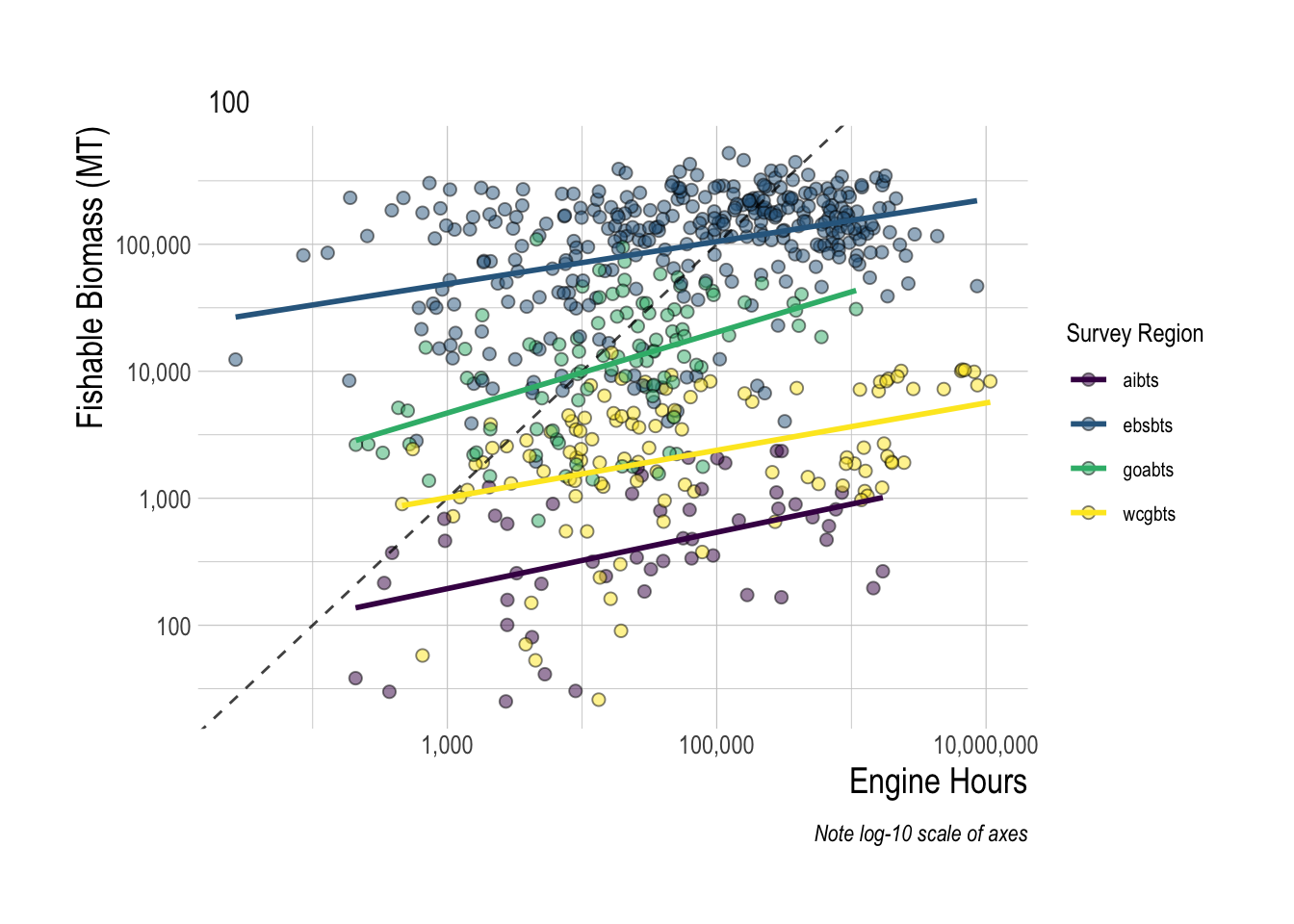
Figure 1.6: Total fishing hours plotted against fish revenue density. Available revenue is calculated as the sum of the densities of each species times their respective ex-vessel price. Each point represents a 200km2 area
This coarse data analysis suggests that there may be a relationship between total fishing effort and the value of the fishing opportunity within a region, but certainly not a clear enough relationship to serve as a reliable predictor of fishable biomass. That effort levels alone are not clearly informative is not very surprising. What though do we learn by pairing effort data with locally available catch data to construct a CPUE index? CPUE can, under the appropriate circumstances, serve as an index of relative abundance (Maunder et al. 2006), though it can also fail badly at this task if key assumptions are violated (Hilborn and Kennedy 1992; Harley et al. 2001; Walters 2003). Ignoring complications in interpretation of CPUE for now, to create a GFW derived CPUE index, we pulled catch data for the relevant regions and species from three different databases: the RAM Legacy Stock Assessment Database (Ricard et al. 2012), the NMFS commercial landings database, and the FAO’s capture production database (FAO 2018). Pairing these catch data with the the GFW effort data gives us a timeseries of aggregate CPUE for a given region. We then compared these CPUE trends to trends in biomass provided by the RAM database and from the processed trawl survey used throughout this study. In the Eastern Bering Sea region, if you squint there appears to be some a shared downward trend since 2014 between the CPUE indices and the independent abundance indices (Fig.1.7). But, the GFW derived CPUE indices tell the exact opposite story as the independent abundance indices along the US West Coast (Fig.1.8).
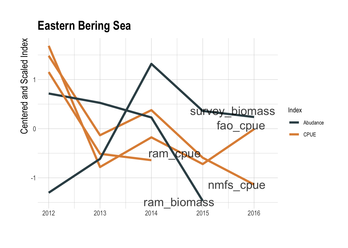
Figure 1.7: GFW derived CPUE (orange) and assessments of abundance (blue) for the Eastern Bering Sea region
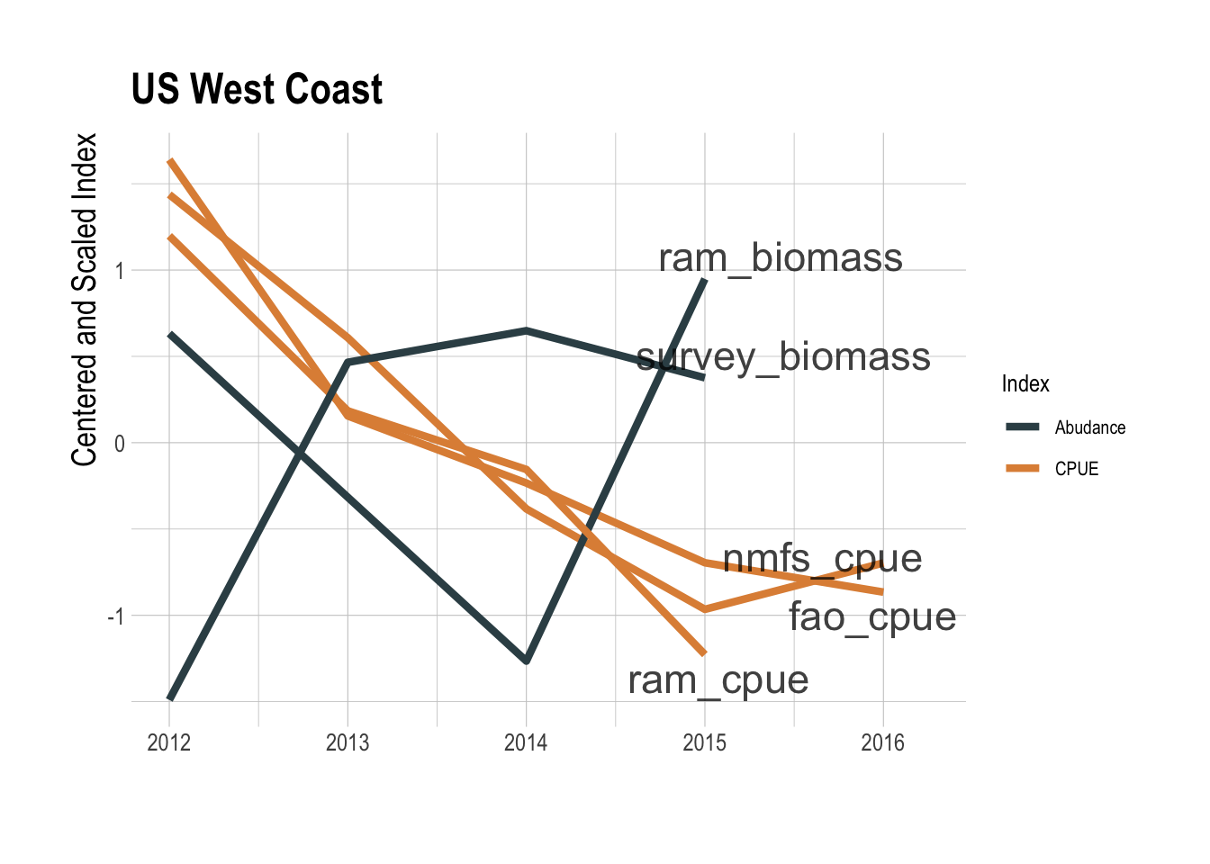
Figure 1.8: GFW derived CPUE (orange) and assessments of abundance (black) for the US West Coast
Turning to the latent variables approach for the linear models, We find no correspondence between the estimated space effects \(\hat{B}\) and the fish biomass estimated from the trawl surveys. This does not mean that such an approach might not work given sufficient data, but with the available covariates either omit too many other important factors besides biomass are being absorbed into the \(\hat{B}\) coefficients, or the survey biomass is a small component of the decision making process for a given fishing location (Fig.1.9).
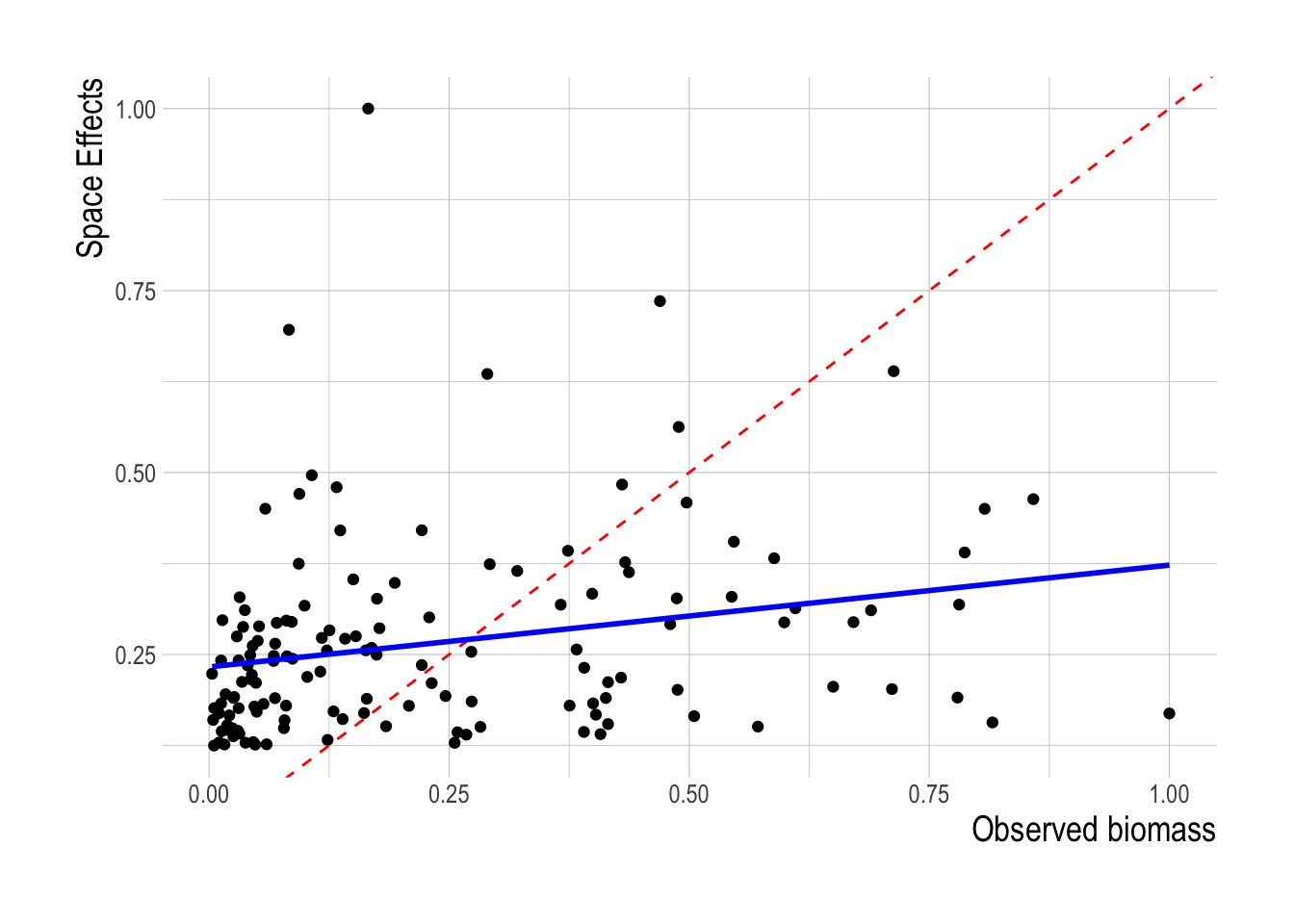
Figure 1.9: Scaled latent biomass coefficients plotted against paired scaled biomass estimates. Red dashed line indicates a 1:1 fit, solid blue line represents a linear model of the two axes
1.4.2 Structural Models
Since raw effort and effort derived CPUE indices do not appear to be valid methods for estimating abundance, we now turn to more detailed modeling approaches to utilize effort data to predict abundance. Our structural modeling approach follows a standard bio-economic framework, as laid out in Miller and Deacon (2016). Miller and Deacon (2016) used a structural modeling approach in part to estimate the quota prices in the US West Coast groundfish trawl fishery individual fishing quota (IFQ) program, using data on logbook reported CPUE, prices, and variable and fixed costs (labor, fuel, etc.). Making the assumption that for an appropriate fleet unit and time period marginal profits are equal in space, Miller and Deacon (2016) then estimate quota prices for different species that, given their other data, rationalize the observed distribution of effort in the fishery. We applie this same theory to our data, but rearranging the equation so that the model now estimates biomass rather than effort. This biomass-predicting structural model shows limited predictive ability within the training set, with R2 within the training data less of 0.13.
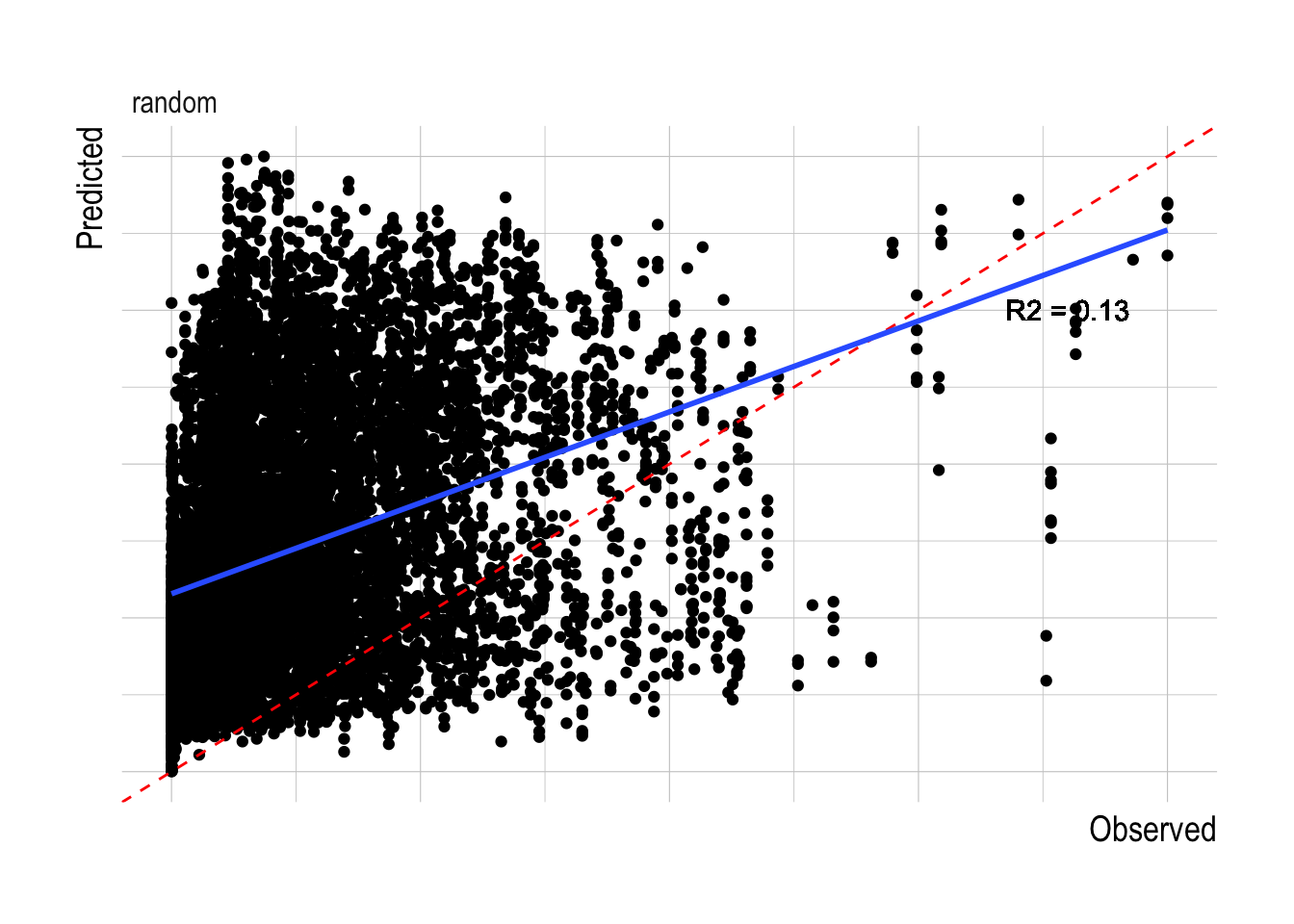
Figure 1.10: Observed vs predicted biomass (A) and R2 values (B) for the fitted structural model. Red dashed line shows 1:1 relationship, blue line a fitted linear model to the observed and predicted values
We can also inverted this idea in the same manner as we did with the linear model, and rather than estimating cost coefficients that explain the observed fish abundance, given observed efforts, estimate cost coefficients and latent spatial parameters representing abundance that explain the observed effort. We estimated this model using a Bayesian hierarchical model implemented in brms (rather than rstanarm since the model is no longer linear). Similarly to the linear model exercise, we found no relationship between the estimated latent spatial abundance coefficients and the estimates of fish abundance provided by the trawl surveys (Fig.1.11).
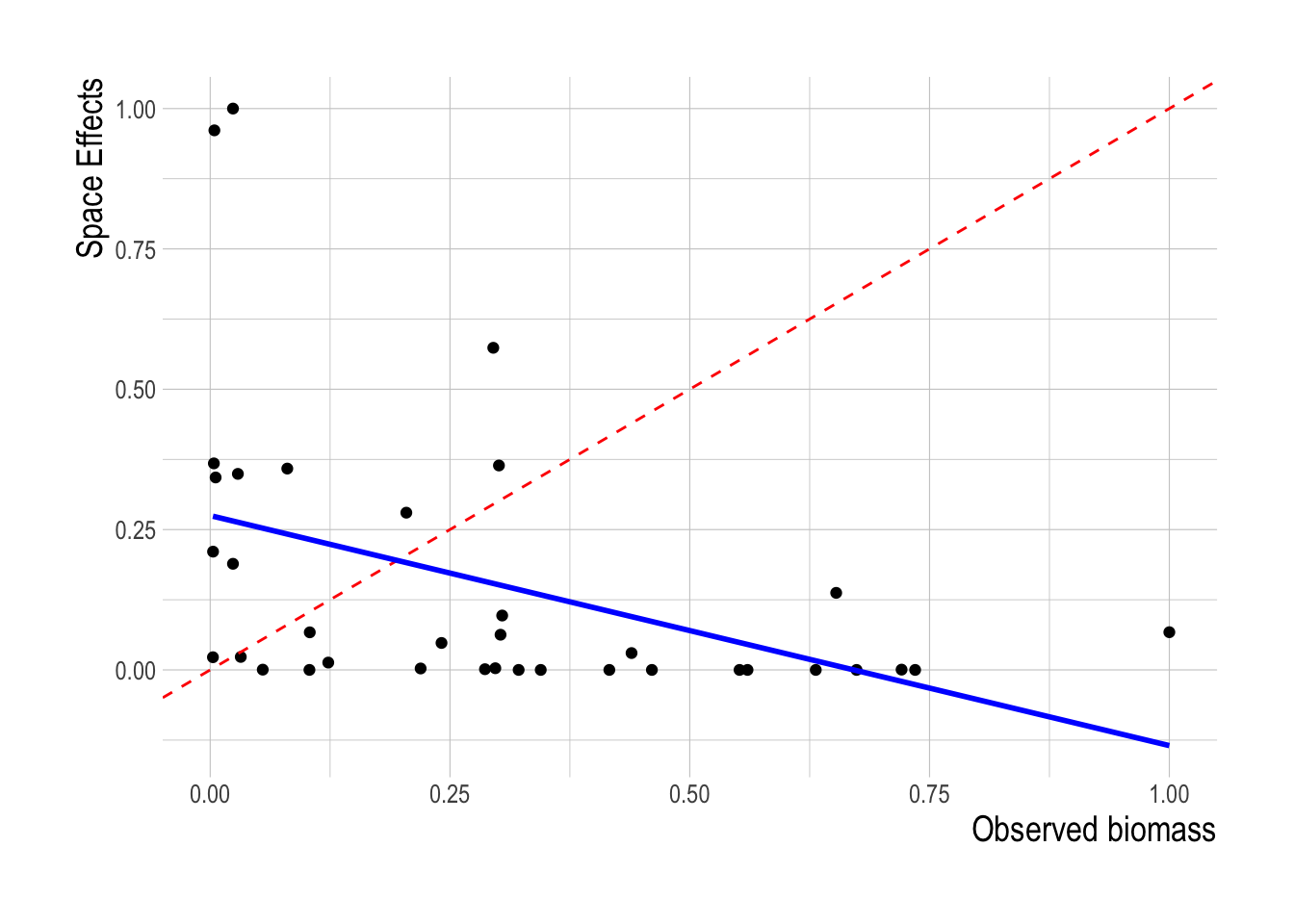
Figure 1.11: Scaled latent biomass coefficients plotted against paired scaled biomass estimates. Red dashed line shows 1:1 relationship, blue line a fitted linear model to the observed and predicted values
1.4.3 Machine Learning Models
Linear and structural models demonstrate little ability to accurately predicting fish abundance using effort data. We turned to machine learning as a final strategy for predicting fish abundance using fishing effort. We tested four different machine learning approaches: random forests (ranger, Breiman 2001), gradient boosted machines (gbm), and multivariate adaptive regression splines (bagged MARS and MARS models). Each of these machine learning models is designed to make use of supplied data to maximize out-of-sample predictive power. However, each model also contains a number of tuning parameters that can only be reliably selected by cross-validation. To that end, we used the caret package in R (Kuhn 2008) to perform two repeats of ten fold cross validation across factorial combinations of candidate tuning parameters, and selected the set of tuning parameters that minimized the out-of-sample root mean squared error (RMSE).
With those tuning parameters in hand, we then utilized the cross-validation routines from those selected tuning parameters to quantitatively compare each of the tuned machine learning models in terms of their out-of-sample predictive power. For each model, we have twenty out-of-sample RMSE estimates. We used the tidyposterior package to fit a Bayesian hierarchical model that, controlling for split effects, estimates the relative effect of each candidate model on out-of-sample RMSE. Based on this analysis, the random forest model (as implemented by the ranger package) has the lowest estimated out-of-sample RMSE. As such, we use the random forest, as implemented by the ranger, as our candidate machine learning model for the remainder of this paper.
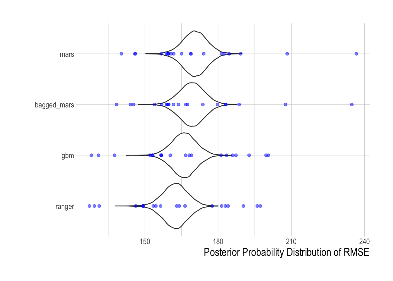
Figure 1.12: Posterior densities of out-of-sample RMSE predicted by tidyposterior
The other decision to be made within the model fitting process is what resolution of data to use within the fitting process. The finest scale effort data pulled from Global Fishing Watch provides the largest sample size, but also potentially increases the noise in the data. Aggregating the data at coarser spatial aggregations decreases sample size but also may decrease noise. We tested the models at three different spatial resolutions, raw, at 25km2 resolution, and 100km2 resolution. The 100km2 resolution had the highest R2 for the training data, and so we will use that as our default resolution for this analysis (Fig.1.13). Using the 100km2 resolution data, the random forest has substantially greater predictive ability within the training data split than any of the linear or structural approaches, with a median R2 across the training splits of over 0.5 (though the model also appears to be positively biased, Fig.1.14).
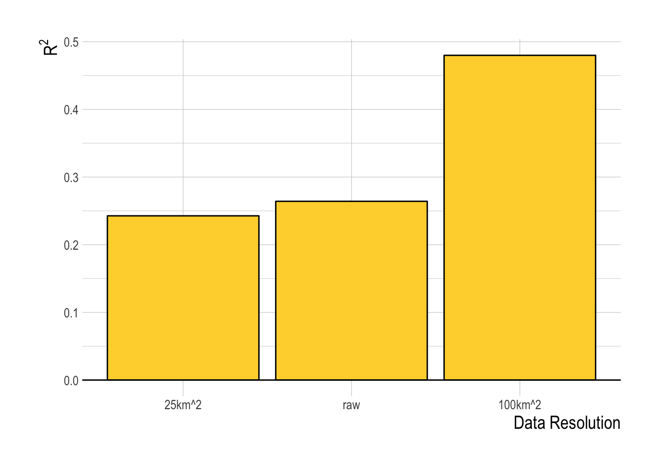
Figure 1.13: Training data R2 for the random forest (ranger) model at three evaluated spatial resolutions of the data
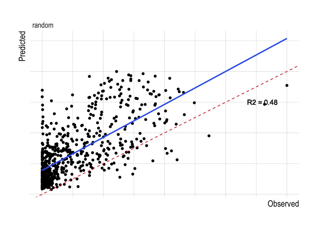
Figure 1.14: Observed vs predicted biomass for the fitted random forest models across different evaluated data splits. Red dashed lines indicates 1:1 fit, blue line a fitted linear model to the observed and predicted values
We can repeat this same resolution procedure to perform one final performance comparison between the random forest and structural models. For each model, we fit the model using the finest resolution data, and then aggregated predictions up to coarser resolutions (Fig.1.15-A), and refit the model itself using coarser resolution data (Fig.1.15-B). Using coarser resolution data in the model fitting process improves the predictive power of the structural models somewhat, but the random forest still outperformed the structural approach across all spatial resolutions. This analysis confirms that a spatial resolution of 100-200km2 appears to be ideal in terms of balancing noise reduction with sample size.
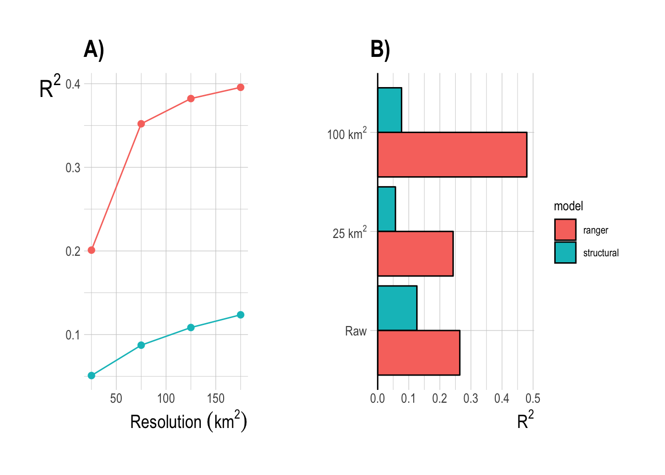
Figure 1.15: Training set R2 from aggregating results of model fit on finest resolution (A) and fitting the model at coarser resolutions (B)
1.4.4 Value of Information
So far, the model with the greatest predictive power, as measured by the R2 of the model within the training data, is a random forest model trained on a random subset of the available data aggregated at a 100km2 resolution. Under those conditions, we see training set R2 in the vicinity of 0.5. Is this good? Models such as Costello et al. (2012) report R2 values near 0.4, so 0.5 would appear to be a respectable value. However, the explicit purpose of this analysis is to determine the value of the effort data supplied by Global Fishing Watch for estimating fish biomass To get at this, we can compare the predictive power of the Global Fishing Watch based model to an alternative model for estimating fish abundance using different sources of information. There are clear theoretical reasons to believe that fishing effort should respond to and affect fish biomass. However, the environment also plays a substantial role in driving fish dynamics, both in abundance and spatio-temporal distribution (Szuwalski and Hollowed 2016; Munch et al. 2018). A model of fish abundance based solely on environmental drivers makes at least as much conceptual sense as a model based on effort and fleet characteristics then.
Based on this idea, we pulled globally estimates of chlorophyll concentrations (a measure of primary productivity), along with sea surface temperature, and bathymetry, from the National Oceanic and Atmospheric Administration ERDDAP platform. We paired these data with non-effort based data pulled from Global Fishing Watch (distance from shore, MPA status), since these data are not part of the novel effort data provided by Global Fishing Watch. We then refit the machine learning models (since the structural models require effort data) using only the environmental data, and using both the environmental data and effort data (following identical fitting procedures across all runs). This allows us to assess the change in predictive power (as measured by R2 of the training data) that including effort data provides.
Comparing effort data alone vs environmental data alone, we see that the relative value of information of the effort data is in fact negative. Meaning, the environment-alone model substantially outperformed, in terms of training data R2, the effort-alone model. If the effort data by themselves are not as predicatively useful as environmental drivers, are the effort and environmental data together worth more than the sum of their parts? Our results suggest that in fact they are not; combining the effort data with the environmental data provides nearly identical performance to using just the environmental data (Fig.1.16).
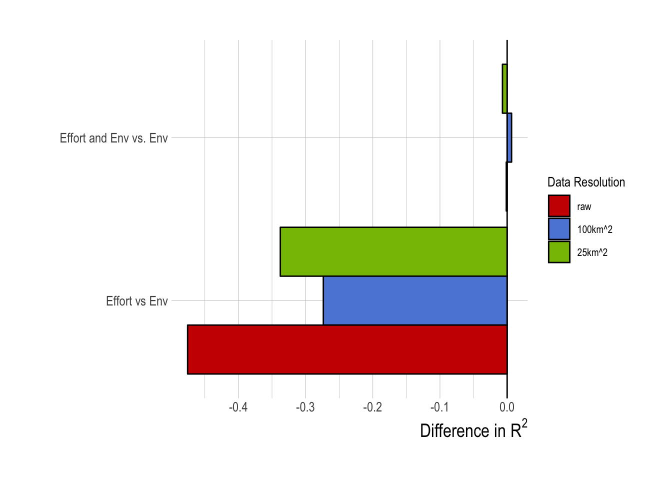
Figure 1.16: Differences in R2 of tuned random forest model with effort data relative to R2 obtained from only using environmental (env) data (negative implies worse performance than environmental data only)
1.4.5 Confrontation with Testing Data
The preceding steps have determined that the best model, in terms of training data R2, is a random forest fitted with data aggregated at the 100km2 resolution, using both environmental and effort data. The end goal of this model though is not to predict data within the training set; instead, we would hope to use this model to help us understand fish abundance in situations outside of the data used to train the model, either in space (i.e. new locations) or time (periods not covered by the trawl surveys). As discussed earlier, the decision of what model to use must be made by examining the training data (and splits of the training data) alone. Now that we have used the training data to select a model that the evidence suggests will have the highest chance of performing well out of sample (remember that even within the training data, the random forest looks to avoid overfitting), we can now confront our selected model with the held out testing data. We also include the structural models in this comparison to see if the structural assumptions of these models provide an advantage in out-of-sample prediction, though we have not provided the structural model with the same built-in resistance to overfitting to the training data that the machine learning models benefit from.
The predictive performance of our candidate models against the testing data indicate that the decisions based on the training data were well founded. Inclusion of the effort data did not improve the performance of the models on the testing data, and across nearly all cases the machine learning approaches still outperformed the structural models. Looking at just the random test-training splits then, our results would seem to show that a random forest based largely on environmental drivers is a good out-of-sample predictor of fish abundance. Before we start replacing stock assessments with remote sensing of environmental drivers though, we should look at the out-of-sample performance of the models trained on other data splits (Fig.1.17).
Under the “historic” data split, the training split consists of observations from 2012-2013 and the testing split from 2014-2017. Under this split the performance from the training to the testing split drops off much more dramatically than under the random split, showing that predicting new years is a much more challenging task for the model than filling in gaps within a year. Similarly, we see that a model trained on data off of the Washington/Oregon coast alone is almost completely useless as a predictor of fish biomass off of California.
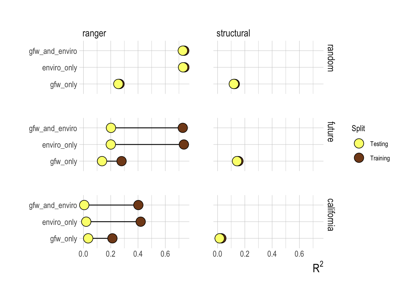
Figure 1.17: R2 for testing and training splits across candidate variables and models. Columns represent the ranger (random forest) and structural models, rows are test-training splits, where row name indicates the dataset that was held out for testing
Our analyses so far have focused on R2 values as a measure of predictive accuracy. These R2 values represent the fraction of the variation in spatio-temporal fish abundance explained by each of our models. A model with an R2 of say 0.9 would then likely be very good at both replicating both a map of abundance and a plot of abundance over time (made up of aggregating each of the individual location estimates over time). However, it is entirely possible that a model with a poor predictive R2, while unlikely to do a good job of capturing the spatial distribution of abundance, may still provide a reasonable index of the trend in abundance (if each point is off but all on average reflect a common trend).
To explore this idea, we can examine the “future” testing case more carefully. In this data split, we trained all models on data from 2012-2013, and used the fitted coefficients from this period to predict data from 2014-onward. Using this model, we then summed the total biomass predictions across space to create a total estimate of biomass within a survey region and a given year. Examining the results, we see that all of the models show evidence of capturing aspects of the trend in the 2014-onward period. In the Eastern Bering Sea region in fact, the random forest model using only Global Fishing Watch data appears to do a slightly better job of representing the trend in the observed abundance trends, though with only four data points it is not wise to make any definitive statements about this, especially since this pattern is reversed in the West Coast data, where use of the environmental data provides better projected predictions (Fig.1.18).
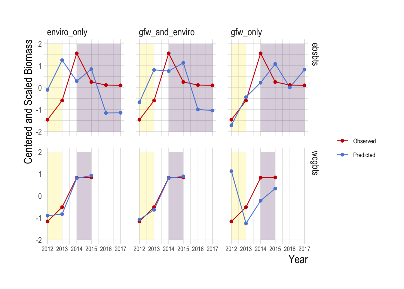
Figure 1.18: Observed (red) and predicted (blue) centered and scaled total biomass estiamtes over time. Yellow regions indicate data used in the training model, purple shaded regions data held out from the model training. Note that in order to avoid problems with increasing spatial coverage in the GFW data, only locations consistently present over the entire timespan of the data are included
1.5 Discussion
The goal of this project was to determine the value of the effort data provided by Global Fishing Watch in estimating fish abundance in space and time. We accomplished this by first determining through a set of fitting routines (models, tuning parameters, resolution) the model that, given the training data, appeared to provide the highest likelihood of performing well, in terms of predictive ability, both in and out of sample. This process found a random forest tuned on 100km2 spatial resolution data to be the “best” model. From there, we were able to estimate the value of information of the effort data by comparing the predictive power of the selected model using effort data, as compared to the same selected model using only non-effort based data. This analysis showed that the effort data provides little predictive power beyond that provided by the non-effort data alone.
That the machine learning models outperformed the liner and structural models comes as no surprise: machine learning models are designed explicitly for prediction and should be expected to do well at the task. However, they have two central weaknesses that made the evaluation of alternative predictive models important. The first is that they lack any structural assumptions, and therefore are relatively un-interpretable. Structural models, such as the bio-economic approach taken here, require assumptions about specific functional forms, but as a result provide a means for rationalizing results, e.g. by providing parameter estimates that can be evaluated and interpreted using statistical methods and theoretical knowledge (e.g. the meaning of a cost coefficient can be understood and our confidence in the value of that coefficient estimated). All else being equal, we would clearly prefer to have an interpretable model than a black box. To that end, when prediction is the objective, we can estimate the “cost” of that interpretability by comparing the predictive ability of a machine learning approach that maximizes predictability of at the expense of interpretability to a structural model that seeks to maximize the likelihood of the data conditional on its assumptions. While, during the training phase, the structural model is unlikely to outperform the machine learning approach, if it comes close, the price in predictability may be well worth the gain in interpretation. In our case though, the machine learning approach so outperformed the structural approach that they cannot be outweighed by the interpretability of the structural approach. This does not mean that the broad concept of the ideal-free distribution that is at the core of the structural model is inherently incorrect, but that that particular model as implemented here is not suitable for the aggregation of the data as they stand. It is entirely possible that finer resolution effort and abundance data (e.g. the logbook data utilized in Miller and Deacon (2016)) would produce better performance from the structural model. But, our results show that a structural bio-economic modeling approach is not appropriate for using the effort data supplied by Global Fishing Watch to estimate fish abundance.
Vastly out-of-sample prediction is a second major problem with machine learning models, and the random forest model selected through this process in particular. A properly specified and estimated structural model provides a clear process for predicting outcomes in situations that are far outside of the scale of the training data. Suppose for example that the structural model is a simple linear regression with a slope and intercept, trained on one independent variable on the range one to twenty. If we then confront our fitted model with a new independent datapoint with value of 1,000, our estimated slope and intercept allows us to easily provide a prediction for this new data point (though of course the accuracy of this prediction will depend on the accuracy of our model). A random forest is able to do this process as well, but lacks a clear mechanism for doing so. A random forest works by fitting a forest of regression trees, each of which, in the case of continuous predictors, break the predictors into a series of bins. Therefore, the predicted outcome for a dependent variable 100 times greater than any value used in the training value will be more or less the same as the prediction for the largest value of the dependent value in the training data (i.e. the new data point will fall into the “greater than some cutoff” bin). If there is some continuous relationship between the dependent variable and the outcome, this prediction may be severely biased. Because of that, machine learning models such as random forests are best at “filling in the gaps” for data fitting within a defined parameter space, and can struggle when fit on one parameter space and applied to a vastly different parameter space.
We checked for the possibility of this problem by, post selection of the random forest model, examining the predictive ability of that model on both the testing data and the held out training data. Our results show that this flaw of random forests is indeed a problem here: the model does very well at predicting “out of sample” points that are simply random omissions from the complete database. A model trained on the years 2012-2014 and used to predict 2015-2017 (the “future” training-test split) performs worse than the random split, and a model trained on Washington/Oregon data and used to predict California losses roughly half of its predictive power. However, the structural model was still not able to outperform the machine learning approach in these out-of-sample cases. These results show that there are predictable relationships between fish biomass and environmental, and to a lesser extent effort, data, but that these relationships do not easily export to new time periods or locations.
What should we make of the relative lack of predictive value of the effort data, as compared to the environmental data? It is critical to note that this is not to say that the effort data alone does not have predictive power, at least within the rough survey region and time period on which the models are trained. R2 values for a random forest using only GFW data trained on a random subset of the data to predict fish biomass were near 0.5, both for the training and testing splits; the effort data alone are capable predictors. But, if the question is what additional predictive power do these effort data provide us that we could not have obtained from other data streams, such as environmental data, the answer is not much. We do see closer performance of the effort based and environment based models when comparing their ability to predict trends in abundance, as opposed to overall fit (Fig.1.18). This may suggest that effort data supplied by GFW may be more indicative of overall trends in abundance than the exact spatial distribution of abundance However, given the very short time-span over which both effort and abundance data are available, we cannot draw definitive conclusions about the ability of these models to predict trends at this time.
While the effort data’s lack of value in predicting fish is not the result that we hoped for, it is not surprising for two reasons. The first is that this is simply an indication of the long-understood challenges of using effort data alone to make meaningful inferences on the status of fish stocks: more fishing might mean abundant fishing grounds or over-exploited locations where the fishing is cheap. While machine learning approaches may be able to disentangle some of these factors within a region, a relationship between fishing and effort fitted in one region is unlikely to export to a new region or time. A second and more interesting reason though may lie in the nature of the information used by fishermen to make their decisions. While many bio-economic modeling exercises assume perfect knowledge of the location and amount of fish stocks for simplifying reasons, in reality of course the choice of where and how much to fish is an uncertain and complicated process, based on objectives, risk tolerance, past experience and shared knowledge. Part of that decision making process is directly related to observing and reacting to the precise type of environmental drivers included in this analysis. Fishermen understand the preferred depth and temperature contours of their target species, and areas of substantial upwelling, often marked by increased chlorophyll concentrations, have long been known to be productive fishing grounds. So, while the model hypothesized that combinations of environmental and effort data might provide a signal worth more than the sum of their parts, our results suggest in fact with regards to predicting biomass, the effort data are a noisier reflection of the environmental data, but further muddied by the myriad other factors affecting fishing decisions, including costs, regulations, experience, and safety.
The effort data provided by Global Fishing Watch present a novel and massive influx of information that shed light on a variety of different factor affecting our oceans, including the footprint of global fishing (Kroodsma et al. 2018) to the estimates of the profitability of different fishing regions (Sala et al. 2018). This project evaluated the extent to which these data could be used to improve fisheries management by helping estimate fish abundances associated with different effort patterns. We found that these effort data can be used for predicting fish biomass, but that a) the manner in which effort is related to abundance, at least at these aggregated resolutions of multiple gears and multiple species, is poorly described by classical bio-economic models, and that b) while machine learning models were able to provide much greater predictive power, the effort data provided little additional predictive value over other globally available environmental datasets. Further work utilizing effort data derived from Global Fishing Watch in stock assessment will need to find ways of more closely matching effort data with their targeted species, or shift attention from using effort as an indicator of biomass towards using it as a prior on the evolution of fishing mortality rates.
References
Ricard, D., Minto, C., Jensen, O.P. and Baum, J.K. (2012) Examining the knowledge base and status of commercially exploited marine species with the RAM Legacy Stock Assessment Database. Fish and Fisheries 13, 380–398.
Hordyk, A., Ono, K., Valencia, S., Loneragan, N. and Prince, J. (2014) A novel length-based empirical estimation method of spawning potential ratio (SPR), and tests of its performance, for small-scale, data-poor fisheries. ICES Journal of Marine Science: Journal du Conseil, fsu004.
Rudd, M.B. and Thorson, J.T. (2017) Accounting for variable recruitment and fishing mortality in length-based stock assessments for data-limited fisheries. Canadian Journal of Fisheries and Aquatic Sciences, 1–17.
Costello, C., Ovando, D., Hilborn, R., Gaines, S.D., Deschenes, O. and Lester, S.E. (2012) Status and Solutions for the World’s Unassessed Fisheries. Science 338, 517–520.
Costello, C., Ovando, D., Clavelle, T., et al. (2016) Global fishery prospects under contrasting management regimes. Proceedings of the National Academy of Sciences 113, 5125–5129.
Rosenberg, A.A., Kleisner, K.M., Afflerbach, J., et al. (2017) Applying a New Ensemble Approach to Estimating Stock Status of Marine Fisheries around the World. Conservation Letters, n/a–n/a.
FAO (2018) The State of World Fisheries and Aquaculture 2018: Meeting the sustainable development goals, (The state of world fisheries and aquaculture). FAO, Rome, Italy.
Anderson, S.C., Cooper, A.B., Jensen, O.P., et al. (2017) Improving estimates of population status and trend with superensemble models. Fish and Fisheries 18, 732–741.
Pauly, D., Hilborn, R. and Branch, T.A. (2013) Fisheries: Does catch reflect abundance? Nature 494, 303–306.
Kroodsma, D.A., Mayorga, J., Hochberg, T., et al. (2018) Tracking the global footprint of fisheries. Science 359, 904–908.
Gordon, H.S. (1954) The economic theory of a common-property resource: The fishery. The Journal of Political Economy 62, 124–142.
Hardin, G. (1968) The Tragedy of the Commons. Science 162, 1243–1248.
Ostrom, E. (1990) Governing the Commons: The Evolution of Institutions for Collective Action. Cambridge University Press.
Ostrom, E. (2009) A General Framework for Analyzing Sustainability of Social-Ecological Systems. Science 325, 419–422.
Grafton, R.Q. (1996) Individual transferable quotas: Theory and practice. Reviews in Fish Biology and Fisheries 6, 5–20.
Cancino, J.P., Uchida, H. and Wilen, J.E. (2007) TURFs and ITQs: Collective vs. Individual Decision Making. Marine Resource Economics 22, 391.
Deacon, R.T. and Costello, C.J. (2007) Strategies for Enhancing Rent Capture in ITQ Fisheries.
Costello, C. and Polasky, S. (2008) Optimal harvesting of stochastic spatial resources. Journal of Environmental Economics and Management 56, 1–18.
Kaffine, D. and Costello, C. (2008) Can spatial property rights fix fisheries? Working paper.
Wilen, J.E., Cancino, J. and Uchida, H. (2012) The Economics of Territorial Use Rights Fisheries, or TURFs. Review of Environmental Economics and Policy 6, 237–257.
Grainger, C.A. and Costello, C. (2016) Distributional Effects of the Transition to Property Rights for a Common-Pool Resource. Marine Resource Economics 31, 1–26.
Squires, D., Maunder, M., Allen, R., et al. (2016) Effort rights-based management. Fish and Fisheries, n/a–n/a.
Butterworth, D.S. (2007) Why a management procedure approach? Some positives and negatives. ICES Journal of Marine Science: Journal du Conseil 64, 613–617.
Punt, A.E., Butterworth, D.S., Moor, C.L. de, Oliveira, J.A.A.D. and Haddon, M. (2016) Management strategy evaluation: Best practices. Fish and Fisheries 17, 303–334.
Nielsen, J.R., Thunberg, E., Holland, D.S., et al. (2017) Integrated ecological–Economic fisheries models—Evaluation, review and challenges for implementation. Fish and Fisheries, n/a–n/a.
Sugihara, G., May, R., Ye, H., Hsieh, C.-h., Deyle, E., Fogarty, M. and Munch, S. (2012) Detecting Causality in Complex Ecosystems. Science 338, 496–500.
Prince, J. and Hilborn, R. (1998) Concentration profiles and invertebrate fisheries management. In: Proceedings of the North Pacific Symposium on Invertebrate Stock Assessment and Management. Can. Spec. Publ. Fish. Aquat. Sci. 125. (eds G.S. Jamieson and A. Campbell). NRC Press, Ottawa, Ontario, Canada, pp 187–196.
Hilborn, R. and Kennedy, R.B. (1992) Spatial pattern in catch rates: A test of economic theory. Bulletin of Mathematical Biology 54, 263–273.
Smith, T.D. (1994) Scaling fisheries: The science of measuring the effects of fishing, 1855-1955. Cambridge University Press.
Furness, R.W. and Camphuysen, K.(.J.). (1997) Seabirds as monitors of the marine environment. ICES Journal of Marine Science 54, 726–737.
Thorson, J.T., Shelton, A.O., Ward, E.J. and Skaug, H.J. (2015) Geostatistical delta-generalized linear mixed models improve precision for estimated abundance indices for West Coast groundfishes. ICES Journal of Marine Science: Journal du Conseil 72, 1297–1310.
R Core Team (2018) R: A Language and Environment for Statistical Computing.
Kuhn, M. and Johnson, K. (2013) Applied Predictive Modeling. Springer New York, New York, NY.
Thorson, J.T., Fonner, R., Haltuch, M.A., Ono, K. and Winker, H. (2016) Accounting for spatiotemporal variation and fisher targeting when estimating abundance from multispecies fishery data. Canadian Journal of Fisheries and Aquatic Sciences, 1–14.
Melnychuk, M.C., Clavelle, T., Owashi, B. and Strauss, K. (2016) Reconstruction of global ex-vessel prices of fished species. ICES Journal of Marine Science: Journal du Conseil, fsw169.
Miller, S.J. and Deacon, R.T. (2016) Protecting Marine Ecosystems: Regulation Versus Market Incentives. Marine Resource Economics 32, 83–107.
Vermard, Y., Marchal, P., Mahévas, S. and Thébaud, O. (2008) A dynamic model of the Bay of Biscay pelagic fleet simulating fishing trip choice: The response to the closure of the European anchovy (Engraulis encrasicolus) fishery in 2005. Canadian Journal of Fisheries and Aquatic Sciences 65, 2444–2453.
Kristensen, K., Nielsen, A., Berg, C.W., Skaug, H. and Bell, B.M. (2016) TMB : Automatic Differentiation and Laplace Approximation. Journal of Statistical Software 70.
Bürkner, P.-C. (2017) Brms : An R Package for Bayesian Multilevel Models Using Stan. Journal of Statistical Software 80.
Carpenter, B., Gelman, A., Hoffman, M.D., et al. (2017) Stan : A Probabilistic Programming Language. Journal of Statistical Software 76.
Breiman, L. (2001) Random Forests. Machine Learning 45, 5–32.
Maunder, M.N., Sibert, J.R., Fonteneau, A., Hampton, J., Kleiber, P. and Harley, S.J. (2006) Interpreting catch per unit effort data to assess the status of individual stocks and communities. ICES Journal of Marine Science: Journal du Conseil 63, 1373–1385.
Harley, S.J., Myers, R.A. and Dunn, A. (2001) Is catch-per-unit-effort proportional to abundance? Canadian Journal of Fisheries and Aquatic Sciences 58, 1760–1772.
Walters, C. (2003) Folly and fantasy in the analysis of spatial catch rate data. Canadian Journal of Fisheries and Aquatic Sciences 60, 1433–1436.
Kuhn, M. (2008) Building Predictive Models in R Using the Caret Package. Journal of Statistical Software 28.
Szuwalski, C.S. and Hollowed, A.B. (2016) Climate change and non-stationary population processes in fisheries management. ICES Journal of Marine Science 73, 1297–1305.
Munch, S.B., Giron‐Nava, A. and Sugihara, G. (2018) Nonlinear dynamics and noise in fisheries recruitment: A global meta-analysis. Fish and Fisheries 0.
Sala, E., Mayorga, J., Costello, C., et al. (2018) The economics of fishing the high seas. Science Advances 4, eaat2504.