Chapter 2 Predicting and Detecting the Regional-Scale Conservation and Fishery Impacts of Marine Protected Areas

2.1 Introduction

Marine Protected Areas (MPAs, which we will define here as spatial regions in the ocean in which fishing for species of interest is prohibited, acknowledging that other regulatory definitions of MPAs exist) have a long history in the management of marine resources. Traditional cultures in Oceania utilized (often temporary) MPAs as a sort of “fish bank” for times of need (Johannes 1978). In more recent times, MPAs were first put in place primarily as conservation areas, analogs to terrestrial reserves deigned to protect iconic landscapes such as Yellowstone or Kruger National Parks. However, over time our goals and expectations for MPAs have evolved; we now frequently consider the use of MPAs to both protect marine ecosystems within their boundaries and bolster fish populations and fishing opportunities in their surrounding waters (Gaines et al. 2010).

We have clear and compelling evidence that well enforced MPAs can provide conservation benefits within their borders (Halpern and Warner 2003; Lester et al. 2009; Edgar et al. 2014). As conservation benefits accrue inside an MPA, the MPA can affect the waters beyond their borders through adult or larval spillover, meaning the export of either adult or larval fish from within an MPA’s borders to surrounding waters. Several studies have documented empirical evidence for the existence of adult or larval spillover affecting both abundance and fisheries (Russ and Alcala 1996; McClanahan and Mangi 2000; Stobart et al. 2009; Halpern et al. 2009; e.g. Goni et al. 2010; Kay et al. 2012; Thompson et al. 2017). Given the lack of attention paid by most fish and their larvae to lines on a map, there is no doubt that some degree of spillover occurs from MPAs. The more complex question then is not whether spillover occurs, but what the net effect of spillover is. From a fishery perspective, are spillover benefits sufficient to offset losses in fishing grounds? From a conservation perspective, how much does the buildup of adults inside an MPA increase abundance outside, or does concentration of fishing outside the reserve result in a net loss in regional abundance?

As stakeholders around the world increasingly seek to use MPAs in the marine resource management portfolios, it is critically important that we develop a better understanding of the magnitude and drivers of regional-scale MPA effects. To address this gap, this study examines two critical questions: 1) What do we expect the regional-scale conservation effects of MPAs to be and 2) When (and how) can we expect to detect these effects? We address these questions using a simulation analysis framework to frame the theoretical regional conservation and fishery impacts of MPAs, from which we then develop an empirical assessment of the evidence for regional-level effects of MPAs resulting from a network of closures put in place in the Channel Islands, California, in 2003.

2.1.1 What Does Theory Tell Us?

Before we start, we should define “regional-scale MPA effects” for the purposes of this paper. We define regional-scale conservation MPA effects as the change in total biomass of fish (summing inside and outside of MPAs) relative to the total biomass fish that would have occurred without the MPA In clearer words, how many more or less fish are there throughout the study region as a result of one or more MPAs? Note that this is different from questions such as do MPAs cause an increase of fish inside their borders, or do connected networks of MPAs provide greater benefits than isolated MPAs with equal coverage (???). From the fisheries perspective, we define regional MPA effects as the difference in fishery catches following implementation of an MPA, relative to what the fishery would have caught in the absence of the MPA. Defining “regional” is not a clear-cut exercise. Regional could be defined as a bio-geographic area (e.g. the Channel Islands), or as the range of a interbreeding population (in line with a fisheries definition of a “stock”), or through the range of connectivity of a species through movement. For brevity’s sake, for the remainder of this paper we will refer to the “regional-scale conservation MPA effects” as conservation effects. While the definition of an appropriate region will vary from place to place, the key point here is that we are considering the net effect of MPAs both within and outside of their borders, within a spatial area on which they are capable of having an impact (see Fig.2.1 for an illustration of the regional conservation MPA effect). For the empirical portion of this study, we define “regional” as encompassing the central islands of the Channel Islands National Marine Sanctuary: Anacapa, Santa Cruz, Santa Rosa, and San Miguel.

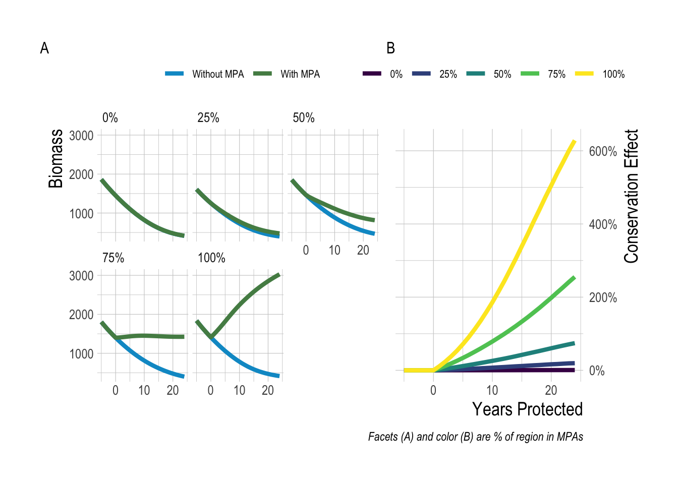
Figure 2.1: Example trajectories of biomass with and without MPAs under a range of MPA sizes (A), and resulting MPA effect (B)

With that definition in mind, what does basic theory suggest should be the magnitude of these regional effects? On one hand, if we imagine a region that has driven its fish populations to near extinction that then places 100% of its waters inside a no-take MPA, we would expect the regional-scale conservation effects to be massive, and in fact to approach infinity (in terms of percentage increase) the closer the “pre MPA” populations approach zero (assuming that the populations are not so depleted as to prevent recovery). On the other hand, If we implement an MPA in place for a lightly fished sedentary species, and in doing so displace a large amount of fishing effort to the waters outside the MPA, it is actually possible to create a net conservation loss. So, this exercise tells us that regardless of almost any other factor, the range of possible regional effects (on a percentage scale) spans the range of of some negative number to positive infinity.

However, within these extremely broad bounds, numerous other factors can act to affect the regional effects of MPAs. These include, but are certainly not limited to, the scale of adult and larval dispersal relative to the size of the MPAs (???; Gaines et al. 2003; Botsford et al. 2008), the strength and timing of density dependence in the population (e.g. pre or post settlement), how overfished the population was pre-MPA, and how fishing activity responds to the implementation of the MPAs (Hilborn and Walters 1992; Gerber et al. 2003, 2005; Hastings and Botsford 2003; Hilborn et al. 2004a,b; Walters and Martell 2004; Gaines et al. 2010). In addition, even for the same total area of MPAs, the location and spacing of the MPAs can have a profound influence on their cumulative impact through habitat and network effects (Costello et al. 2010; Gaines et al. 2010). Broadly, a wide range of theory and modeling exercises indicate that the expected effects of MPAs can vary widely and are extremely context- dependent (Fulton et al. 2015).

At the most “conservation friendly” side of things, we could imagine a group of heavily fished species with limited home ranges as adults, broadcast larvae throughout the region, have post-settlement density dependence, and have a fishing fleet that exits the fishery in proportion to the area protected inside MPAs (e.g. a grouper fishery in which fishing was dependent on a large spawning aggregation). Under these circumstances, the MPAs can be expected to provide a substantial influx of new recruits to the overfished areas outside of the reserve, even as the reserve fills in with adults. At the other end, consider a complex of lightly fished species with relative high adult mobility, pre-settlement density dependence (e.g. at the spawning level, for example a species with specific space and habitat requirements for breeding), and a fishing fleet that concentrates into the remaining fished areas. Under these circumstances, it will be much more challenging for the MPA to provide substantial conservation benefits. Theory then helps us think about the likely regional effects of a given MPA, but outside of these simple cases the cumulative effect of interacting drivers means that the expected regional effects are not analytically solvable or obviously predictable.

2.1.2 What Empirical Evidence Do We Have?

We focus here on evidence of effects of MPAs beyond their borders, see Lester et al. (2009) for a thorough review of within-MPA effects. Many of the studies that explore the effects of MPAs outside of their borders focus on studying gradients of abundance, commonly measured through catch-per-unit-effort (CPUE) or estimated densities along a distance gradient from MPA borders. Presence of negative gradients (decreasing CPUE with distance from MPA border) is taken as evidence of “spillover”, or the export of (generally) biomass from MPAs to their surrounding fished areas

Halpern et al. (2009) conducted a rigorous meta-analysis of empirical evidence for spillover from MPAs. They find that frequent evidence for spillover from MPAs, but at relatively small spatial scales (on average up to 800m from reserve boundaries), though since these studies are in fished system, it is unclear if this distance is reflective of the biological range of spillover, or the intensity of fishing pressure along the border of an MPA. Gell and Roberts (2003) surveyed empirical evidence for adult and larval spillover from MPAs. They documented numerous examples of studies showing decreases in CPUE of adult biomass with distance from MPA borders, commonly attributed to buildup of density inside MPAs and subsequent export of fish biomass, though they also note that evidence for larval spillover is less reported, likely since it is much more difficult to measure than adult biomass (as opposed to an alternative explanation which is that larval spillover happens less than adult spillover).

Russ and Alcala (1996) documents changes in densities or large predatory fish inside and outside of a small marine reserve on Apo Island, Philippines (0.45km long at the time). They report a positive correlation between years of MPA existence and fish densities, but note that up to 8 years of protections were required to detect a significant gradient in fish densities radiating from the reserve borders. Russ et al. (2003) presents a similar study focused on the surgeonfish Naso vlamingii, in which they find dramatic density increases within the reserve, as well as a strong correlational relationship showing catch-per-unit effort of Naso vlamingii decreasing with distance from the reserve boundary.

Similarly, Harmelin-Vivien et al. (2008) assessed gradients in fish density at increasing distances from cores of MPAs as evidence of spillover in the Mediterranean. They report evidence of decreases in biomass densities with distance from MPA borders, though these effects largely dissipated within 100s of meters of MPA boundaries. Vandeperre et al. (2011) conducted a meta-analysis of spillover effects (again measured as CPUE along distance-from-MPA gradients over time) around MPA in Southern Europe. They also document some evidence of declines in CPUE with distance from MPA border, as well as a 2-4% increase in CPUE per year in the fished area following MPA implementation. Guidetti and Sala (2007) finds similar results in the region.

McClanahan and Mangi (2000) measured spillover effects around the Mombasa Marine Park in Kenya. They also provide evidence of negative CPUE gradients with distance from MPA border, but note that these effects are highly affected by habitat, environmental, and management variables. They document the largest effects for moderately mobile species (e.g. surgeonfish)

Several studies have explored the spillover effects of MPAs along the California coast. Starr et al. (2015) and Caselle et al. (2015) both document rapid but variable changes in fish densities related to marine reserve networks in the Channel Islands and along the central California coast. Starr et al. (2015) found evidence that densities inside MPAs had increased on average, but effects were variable, and found little substantial changes in densities in control sites outside the reserves. Caselle et al. (2015) found similar results, documenting faster increases of densities of targeted species inside reserves than outside, but little change in densities in reference sites. Both of these studies then suggest that spillover benefits may be slow (~10 years) to accrue. Kay et al. (2012) reports strong evidence of spillover of adult lobster from MPAs in the Channel Islands. Thompson et al. (2017) reports increases in abundance of the larvae of targeted rockfish species, relative to comparable trends of larval abundance for non-targeted species, following implementation of rockfish-specific MPAs along the California coast.

Taken together, while a large body of literature has examined the theory for regional-scale MPA effects, very little empirical evidence directly tackles the questions “do MPA cause a net change in regional fish biomass, and if so how much”? Nearly all of the empirical evidence of which we are aware measures spillover, which is often equated with regional-scale effects, by quantifying measures such as CPUE along distance gradients from MPA borders. These studies by and large conclude that spillover effects (measured in this manner) are detectable, but a) can be confounded by environmental and management variables and b) often dissipate at distances greater than 1km from a reserve border. While these studies are extremely important contributions to our understanding of regional MPA effects, and regardless of additional challenges with interpretation of CPUE/density gradients as spillover, even properly measured they do not directly address the question of total regional effects of MPAs.

2.1.3 How Can We Detect Regional MPA Effects?

Given that we know that the regional level conservation effects of MPAs can vary dramatically, how can we go about detecting these effects in real systems? Under our definition, the conservation effect reflects the change in abundance resulting from the MPA relative to what would have happened without the MPA. This is a nice definition, but unfortunately is effectively impossible for us to truly observe in nature. For the case of assessing the conservation effects MPAs inside their borders, the gold-standard tends to be before-after-control-impact studies (BACI, as described in ???, analogous to what is commonly referred to as a difference-in-difference analysis in econometrics, as introduced by (???)). In BACI studies, ideally a set of appropriately matched control and “impact” sites are selected, where the “impact” refers to the eventual implementation of MPAs. Measures of species abundance in the control and impact sites are monitored for some period of time pre and post MPA, and the effect of the MPA on the impact sites (i.e. inside the MPAs) is the difference in the trends in the control and impact sites. So, if abundances at both control and impact sites are trending up, but the impact sites are trending up faster than the control sites, this is evidence that the MPA is “working” inside its borders.

While well designed BACI studies are clearly difficult to successfully implement, and subject to their own set of caveats and assumptions, properly implemented they are an effective strategy for robustly estimating within-border MPA conservation effects (assuming critically that the “control” sites are adequately selected, and that for example MPA sites are not systemically more productive than control sites). A review of existing BACI studies in MPAs did not find clear evidence for this type of bias in site selection (and therefore estimated within-MPA effects, Halpern et al. 2004). However, at the regional scale the task of estimating MPA effects becomes much more complicated. Take for example the Channel Islands region off the coast of California (Fig.2.2). The Channel Islands is an ecologically diverse region that supports a range of fisheries. A network of MPAs was implemented in the Channel Islands in 2003, with the express goal of both providing conservation and fishery benefits throughout the region. Fifteen years after their implementation, how can we tell if they successfully caused an increase in fish abundance throughout the Islands? Following the BACI example above, ideally we would like a carbon copy of the Channel Islands that could be kept MPA-free and monitored pre and post MPA implementation in the “treated” Channel Islands. This is of course impossible; we could perhaps envision utilizing nearby regions as controls, e.g. the mainland coastal waters of the Santa Barbara Channel, but this region is quite different than the Channel Islands, and substantial pre-MPA monitoring is lacking for most sites along the Santa Barbara mainland (though see ??? for an example of using different regions as treatment and controls for testing the effect of networks vs disconnected MPAs).

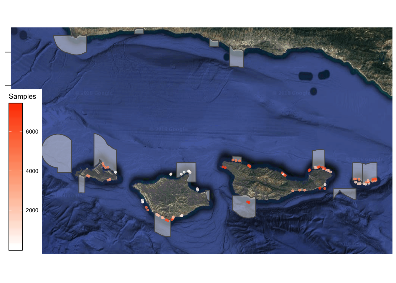
Figure 2.2: Map of study region and sampling locations. Shaded polygons indicate location of MPAs. Points represent sampling locations, and color indicates the number of observations recorded at a given point

As we seek to understand the regional scale effects of MPAs, and as the size of those regions increases, the harder it becomes to find a practical control for the treated region. As a result, it becomes challenging to determine what post-MPA changes throughout the region are attributable to the MPAs and which to other factors. If abundance continues to trend downwards post-MPA, without a control we cannot truly know whether it might have trended down faster without the MPAs. Or, if abundances are trending up, we cannot reliably say that the upward trend is not due to some environmental driver. Regression analysis can help (e.g. statistically controlling for El Niño), but depends on “selection on observables”, meaning that in order to interpret the MPA coefficients as causal, we have to assume that we have included all the correct covariates that might also be correlated with the outcome of interest (in this case abundance of fish). Failure to account for some important variable in our regression can bias results.

We have then two broad options for estimating the regional effect of MPAs in a place like the Channel Islands: We can depend on selection on observables through regression analysis, or we can find an identification strategy. Given the shortcomings of the first approach, we propose an identification strategy building off of Caselle et al. (2015), in which we consider relatively non-targeted species such as Garibaldi (Hypsypops rubicundus) to be “controls” for targeted species such as Kelp Bass (Paralabrax clathratus). Under this strategy, our assumption is that non-targeted species are more or less unaffected by the implementation of MPAs (unlike the targeted species), but that both species are potentially affected by regional environmental trends. In this way, the non-targeted species can serve as our control for environmentally driven shifts in abundance that are not explicitly controlled for in the model (as opposed to a selection on observables approach), allowing us to attempt to better isolate changes in abundance driven by MPAs from changes caused by environmental conditions.

2.2 Results and Discussion

2.2.1 Predicting Regional Effects of MPAs

We used a bio-economic model to simulate the regional effects of MPAs across 20,000 simulated fisheries spanning a wide range of plausible states of nature, including degrees of larval and adult movement, density dependence, fleet dynamics, life history, and pre-MPA exploitation levels, each simulation representing a different state of nature. For simplicity, at this point we focus on single species outcomes, though since we do not model species interactions, fisheries could be together to provide multi-species MPA effects. It is critical to note that we have no current way of assigning probabilities to any of these states of nature, though we have tried to constrain the parameter space to plausible states. Therefore, the results of our simulations suggest simply the number of simulated ways that a given outcome could happen; we do not have any knowledge though if in reality some of these simulated outcomes are individually much more or less likely than others. But, if we assume that the simulated parameter space is a reasonable representation of a range of plausible states of nature, these results provide an indication of the general magnitude of effects that we might expect.

Across this range of scenarios, we see that the median simulated equilibrium regional effect (percentage change in total biomass) was 15%, with a min of -95% and a max of over 200%. We also see that while large percentage increases in biomass can accrue relatively rapidly under some circumstances, increases of over 10% took approximately 10 years to achieve for 50% of the simulated fisheries (Fig.2.3). It is also clear from the simulations that even constrained by reasonable states of nature, a vast array of regional conservation MPA effects are possible. The exact expected regional effect for a given fishery will depend on a complex set of interactions among fishery variables. However, two of the most critical factors affecting the direction and magnitude of the regional effect are the degree of overfishing (displayed in plots as initial depletion, with greater overfishing resulting in higher depletion) present before (and continuing after) MPA implementation, and the size of the MPA, and so we focus on the effects of these two variables on regional MPA effects 15 years after MPA implementation (to mimic the time since implementation of the Channel Islands MPAs at the time of this publication). Across our simulated fisheries, the median 15 year simulated regional effect was 4%. For cases where “small” MPAs (smaller than 25%) were implemented in relatively unexploited fisheries (depletion < 50%), the median regional effect was 0%. For moderate depletion (50% to 75%), MPA sizes from 1% to 50% produced median MPA effects of 3%, while for depletion above 75% the median regional effect from was 80% (Fig.2.4-A). The median regional effect increased with both MPA size and depletion, but it is important to note that the ranges around these median values are extremely wide (Fig.2.4-B). Broadly, the simulation results show that integrating across a broad set of states of nature defined by theoretical drivers of MPA effects, under most simulations the MPAs produced positive effects, though smaller effects were much more likely than large effects. In some instances though, MPAs actually resulted in net regional conservation losses. While factors such as MPA size and pre-MPA depletion are critical drivers, we also show that controlling for these a wide range of outcomes are still possible (Fig.2.4).

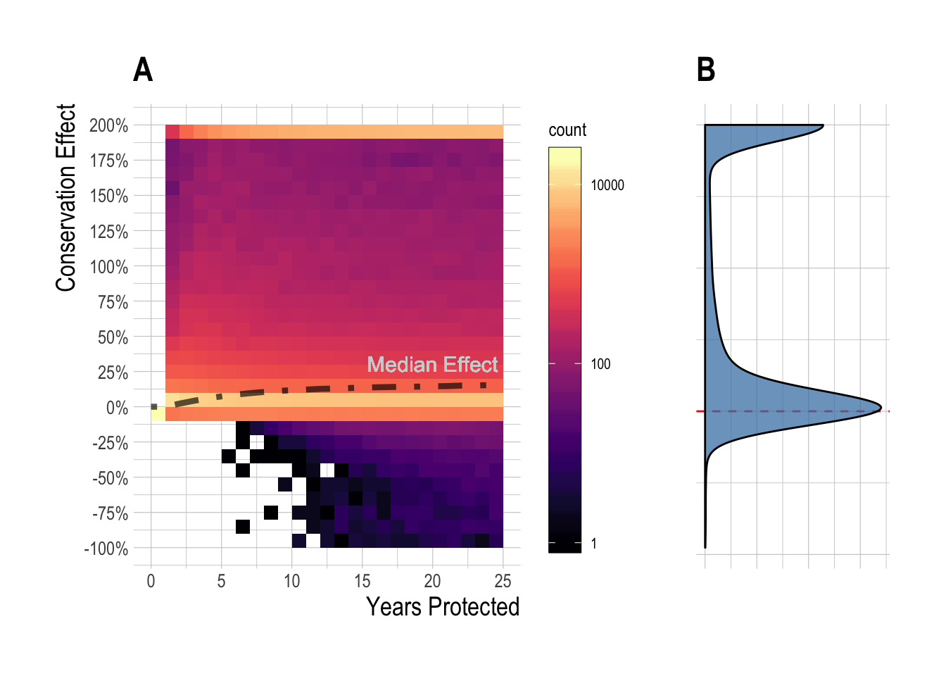
Figure 2.3: Distribution (and median, black line) of simulated regional MPA effects over time (A), and at equilibrium (B). Color indicates number of simulations at a binned effect size at a given time (note log-10 scale of color fill for visual clarity).

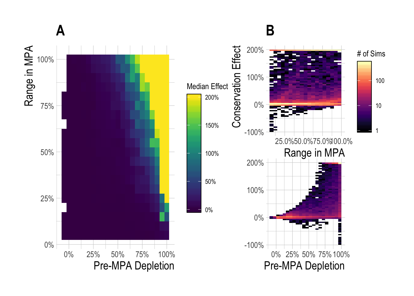
Figure 2.4: Median (A) and range of (B) regional MPA effect after 15 years of protection across a range of pre-MPA depletions and MPA sizes

The percentage change in biomass with and without MPAs is most analogous to the effects that can (in theory) be estimated by our identification strategy (the percentage difference in the density of targeted species relative to the non-targeted species pre and post MPA). However, the percentage change in biomass is a somewhat misleading metric from the perspective of meaningful conservation outcomes. Take for example an extremely depleted scenario where without MPAs a fishery is left with only 2 kg of fish. Suppose then that an MPA brings us up to 6 kg of fish, and that the unfished biomass in this fishery is 1,000kg. While the MPA has produced a 200% increase in fish biomass, this increase is relatively inconsequential given the scale of the population (we have only recovered 0.4% of the unfished biomass), and likely to be very challenging to detect in a real ecological system.

To reflect this, we can repeat the analyses in Fig.??-2.4, but now expressing the change in biomass with and without MPAs as a percentage of unfished biomass for that fishery. Through this metric, we see median equilibrium effect sizes of 2% (Fig. 2.5). Over the 15 year time horizon, our simulations find that MPAs less than 25% produced a median effect of near 0% (Fig. 2.6-A), but again with a wide range around the simulated outcomes outcomes, from -20% to 100% (Fig. 2.6-B).

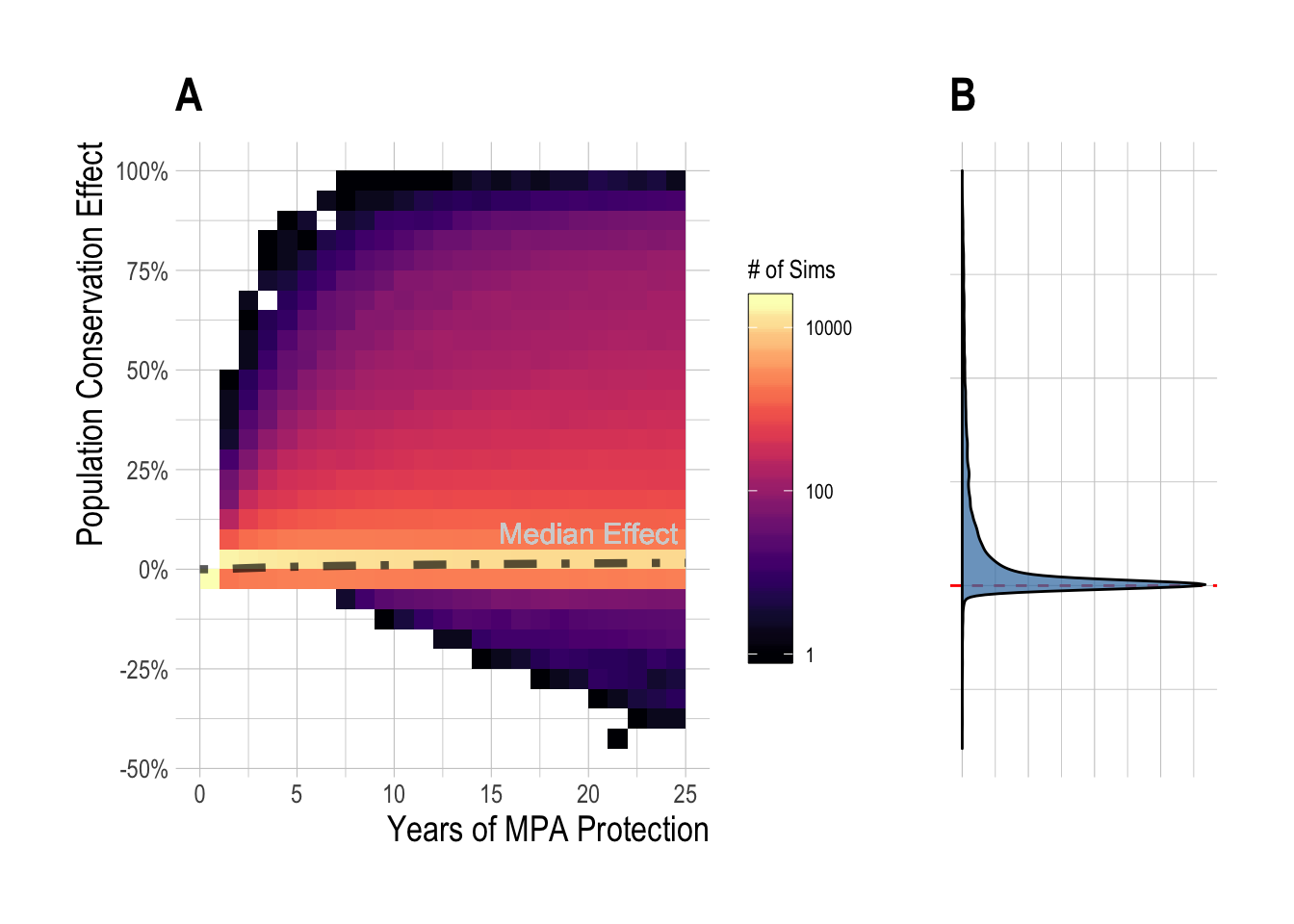
Figure 2.5: Distribution (and median, black line) of simulated regional MPA effects (expressed as percent of unfished biomass) over time (A), and at equilibrium (B)

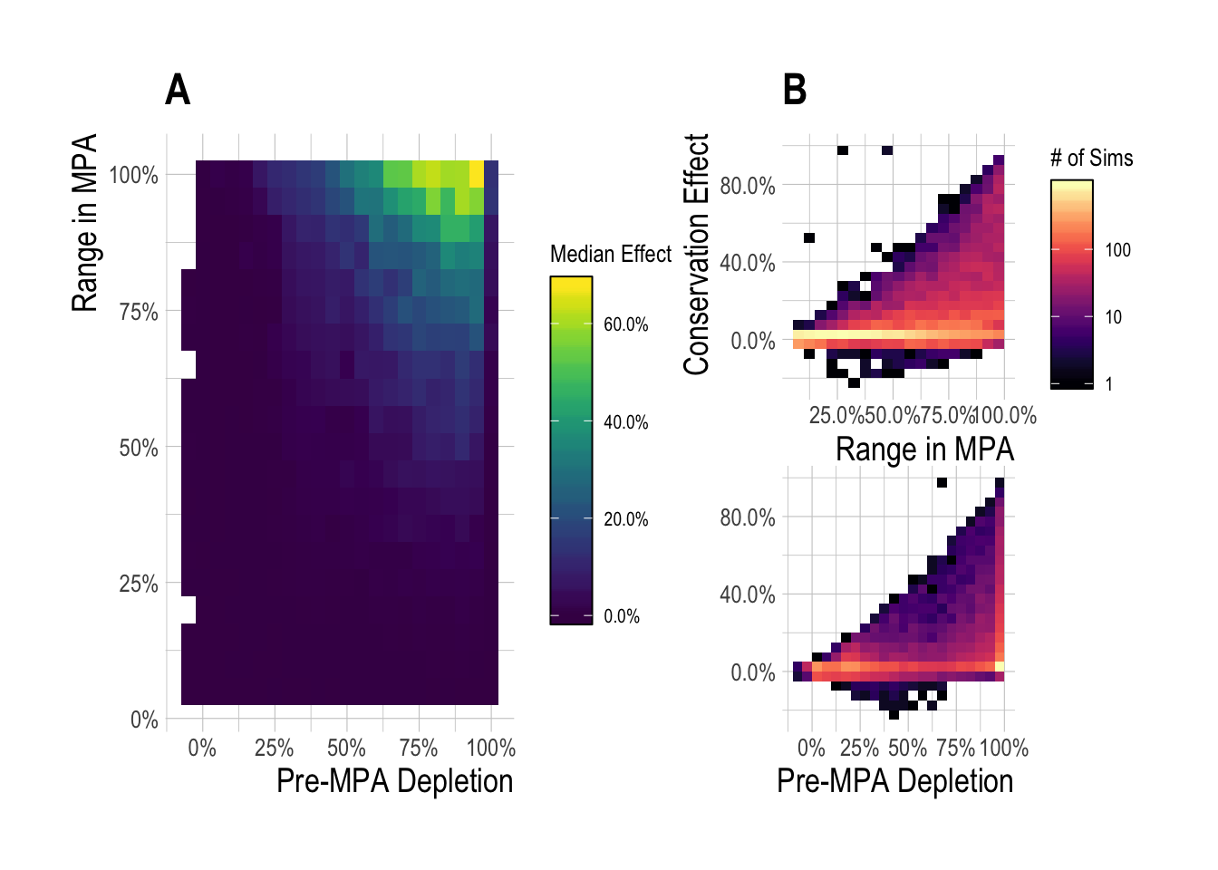
Figure 2.6: Median (A) and range (B) regional MPA effect (expressed as percent of unfished biomass) after 15 years of protection across a range of pre-MPA depletions and MPA sizes

Readers may be especially interested in the simulated scenarios that produced negative MPA effects. The constant-catch fleet model was one of the most important drivers of extremely negative MPA effects, especially when both depletion and MPA size were in the 25-50% range (Fig.2.7). A decision tree analysis conducted using the rpart package through caret confirms that the primary drivers of negative population outcomes are constant-catch dynamics interacting with the size of the MPAs (Fig.2.8). As the name implies, under the constant-catch fleet model fishing communities seek to catch the same amount regardless of the presence of an MPA. While a constant catch greater than MSY is not possible over the long-term under the confines of this simulation framework (the population would crash), over the short-term a constant-catch scenario is not a particularly outlandish idea. Subsistence fisheries may conform to a constant-catch style policy over the short-term, as they seek to ensure the nutritional needs of their community. More industrial fisheries may have pre-arranged purchase orders for levels of catch. Quota managed fisheries may maintain relatively static quota levels until new stock assessments can be completed. The key outcome of these results is that the regional conservation effects of an MPA are critically dependent on fisheries management institutions outside the protected areas; an MPA that would provide large benefits under open-access dynamics may actually harm conservation in a constant-catch scenario.

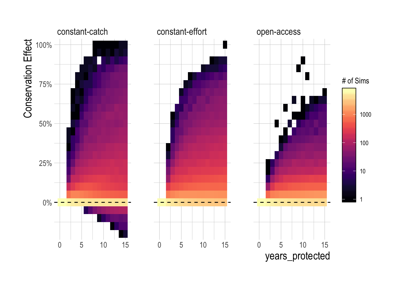
Figure 2.7: Density plot of regional conservation MPA effect by fleet model

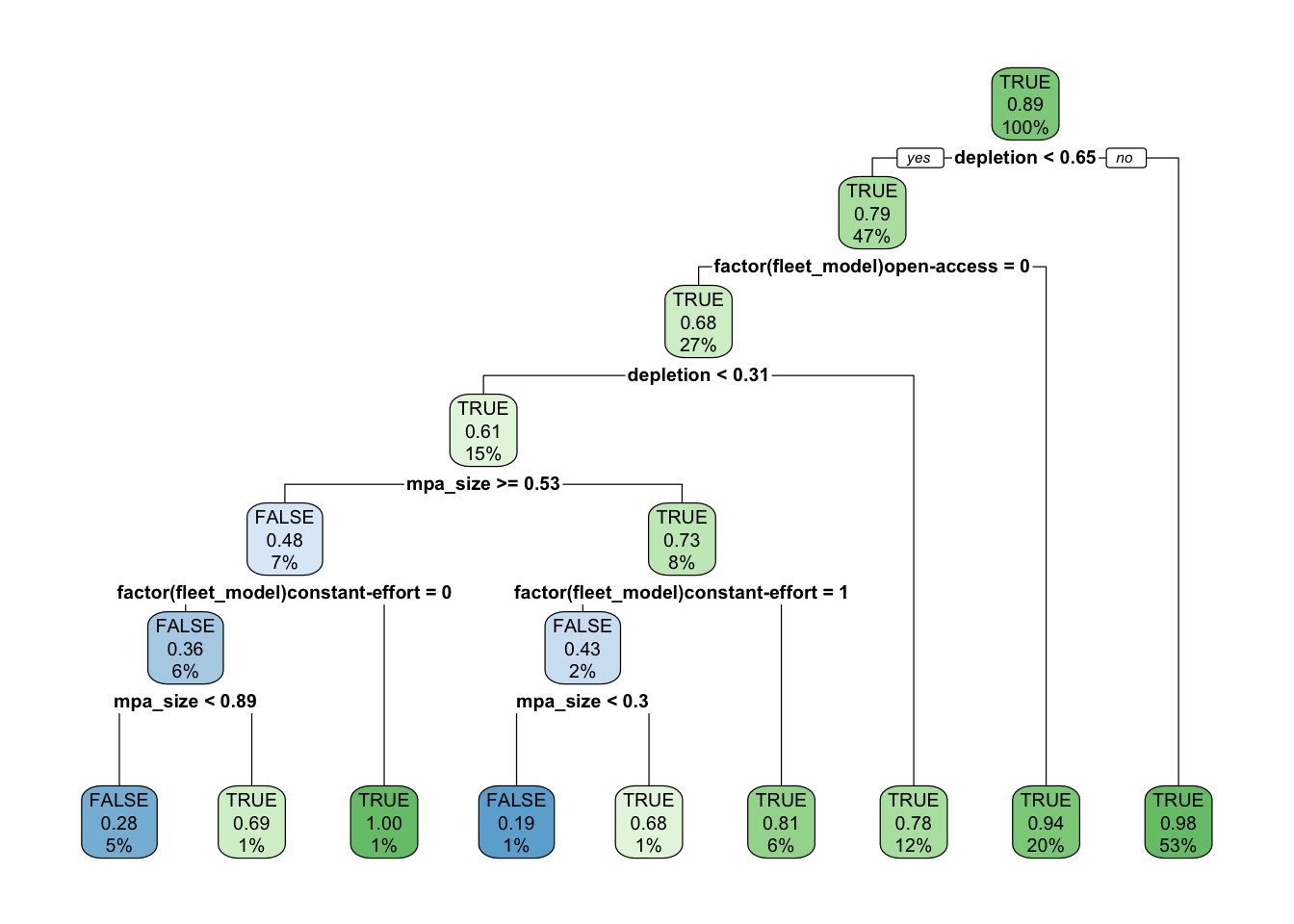
Figure 2.8: Classification tree of positive MPA effects as a function of simulation traits. TRUE indicates that the model predicts there to be a positive regional MPA effect, FALSE a negative effect. Decimal numbers show predicted probability of positive MPA effects, percentages the percent of observations at a given level that fall in that node. Intensity of color is proportional to confidence in prediction (decimal number)

2.2.1.1 Fishery Effects of MPAs

While the emphasis of this particular research project is on predicting and detecting the regional conservation effects of MPAs, the simulation framework that we have constructed also allows us to consider the fishery effects of MPAs, as defined by the percentage gain or loss in total fishery catches following the implementation of MPAs, relative to what the (simulated) fishery would have caught in that scenario without the MPAs. We omit the constant-catch fleet model from this assessment, since by definition (in the short-term at least), catches are the same with or without MPAs (though effort required to obtain those catches, and therefore profits, could be quite different). Similar to the conservation effects, we examined both the median and range of effects as a function of pre-MPA depletion and MPA size. Expressed as a percentage difference in catches with and without MPAs, across our simulated fisheries the median fishery effect for MPA sizes less than 25% and for depletion’s less than 75% (~ B/Bmsy > than 0.6, Assuming Bmsy/K of 0.4) was near 0%. The median fishery effect when depletion was above 80% was commonly near 100%. However, for MPA sizes greater than 25% and for depletion’s less than 75%, the median MPA effect on fishery catches was negative. Pre-MPA depletion was the clearest driver of the magnitude and direction of MPA fishery effects. Meaningful numbers of simulations experienced positive fishery effects only once depletion’s exceeded 50%, with a substantial ramp-up of positive effects after 75%. While both substantial positive and negative effects were possible over a range of MPA sizes, as MPA size passes 50% most simulations start to produce negative fishery effects (Fig.2.9).

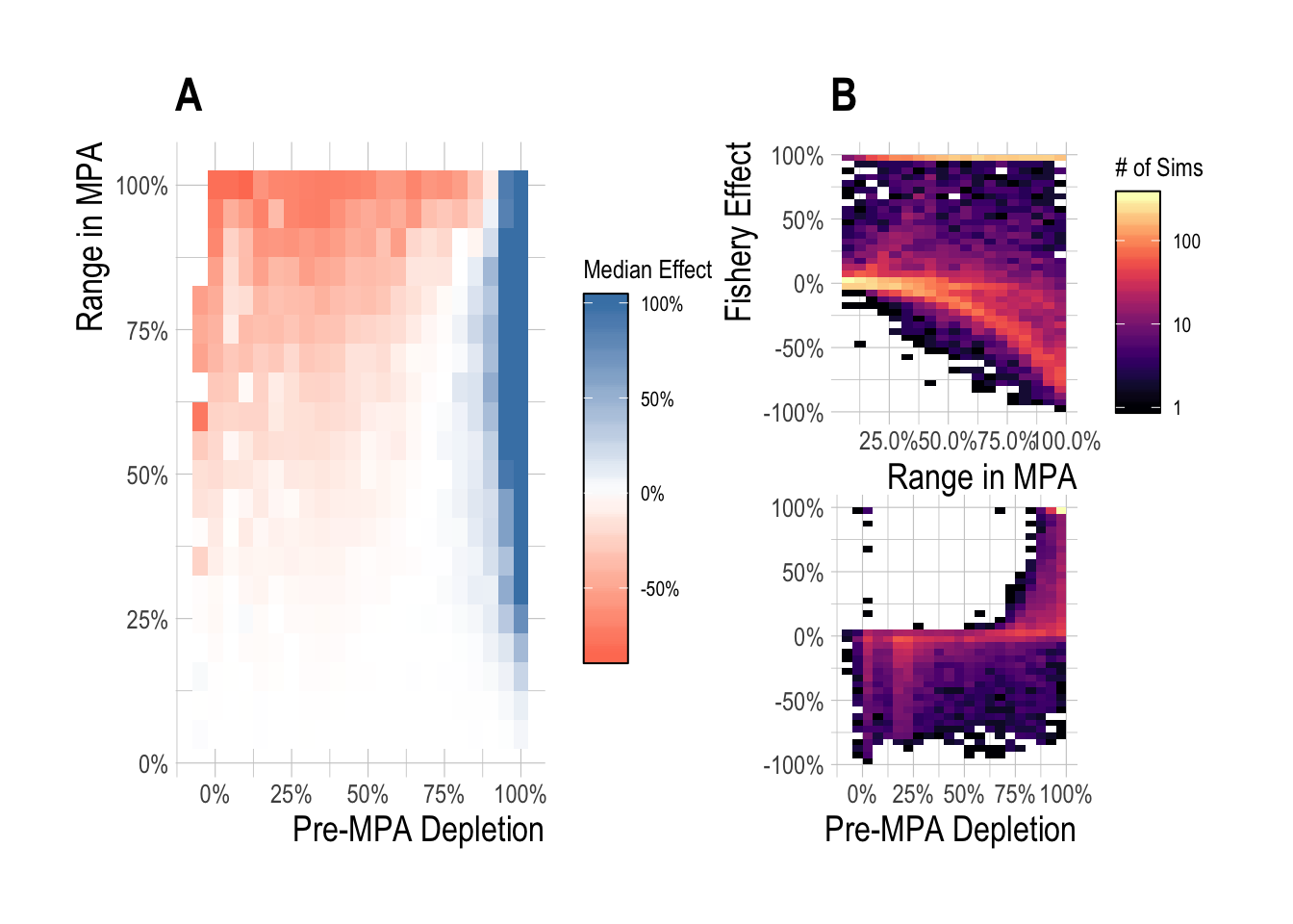
Figure 2.9: Median (A) and range (B) fishery effect (percentage change in catch with and without MPAs) after 15 years of protection across a range of pre-MPA depletions and MPA sizes

Many of the large percentage changes in this analysis can be attributed to very small catches in the absence of MPAs. Catches are generally quite low once a fishery has been collapsed, and so when depletion was near 100%, catches were small, and so a relatively small change in absolute catch following MPA implementation can produce large percentage changes. To address this, we also scaled the differences in fishery catches with and without MPAs by the maximum sustainable yield for that simulated fishery. The fishery effect now reflects the percentage of MSY gained or lost as a result of MPA implementation. The overall trends are similar to the relative change in catch results, but the 15 year effects are more muted, with peak positive effects near 25% and negative effects near -75% (Fig.2.10).

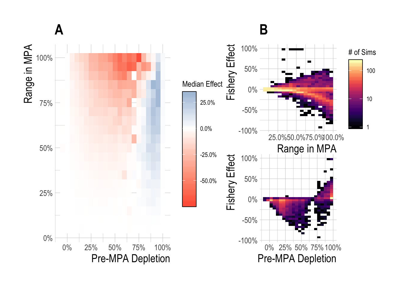
Figure 2.10: Median (A) and range (B) fishery effect (percentage change in catch with and without MPAs relative to MSY) after 15 years of protection across a range of pre-MPA depletions and MPA sizes

2.2.2 Detecting Regional MPA Effects

Theory and simulation testing indicate then that while the regional effects of MPAs can range from strongly negative to highly positive, with the bulk of scenarios producing 0-10% regional conservation effects after fifteen years of protection (though much more negative and much more positive outcomes are certainly possible). Given this, our expectation is that the “true” regional effect will likely be challenging to isolate from the variation of natural systems in and the observation error inherent to any MPA monitoring program. We use data from the Partnership for Interdisciplinary Studies of Coastal Oceans (PISCO) monitoring of the Channel Islands National Marine Sanctuary to test our ability to detect the regional effect of MPAs in a real world context. PISCO conducts visual underwater SCUBA surveys at a variety of rocky-reef and kelp forest sites inside and outside of MPAs throughout the Channel Islands. At the rawest level, the data are counts of finfish in 2cm length bins along a 30m x 2m transect at various sites and depths. These length bins are converted to biomass, and then biomass densities, by converting length to weights using available allometric data and dividing by the transect area. Our goal then is to estimate the effect of the MPAs on these densities of fish throughout the Channel Islands.

Our identification strategy for this case study is to use non-targeted species as our control for unaccounted for environmental trends before and after MPA implementation (which occurred in 2003). The model estimates the difference in the trends between targeted and non-targeted species pre- and post-MPA. We hypothesize that there should be no difference in pre-MPA trends. We fit this model using a hierarchical mixed-effect framework using Template Model Builder (TMB, Kristensen et al. 2016) in R (R Core Team 2018). The model consists broadly of three levels, the first (starting from the “bottom”) being transect-level densities of fish species observed by PISCO, which are standardized into a unit-less index of biomass abundance (which we will refer to as an abundance index from now now), accounting for both probability of detection and expected density as a result of changes in both abundance and covariates such as observer skill (see Maunder and Punt 2004). For the second stage, we break the abundance indices into targeted and non-targeted species (per the classifications in the PISCO data), and estimate the mean trend of each group (targeted and non-targeted) over time. In the third step, we estimate the difference in the mean trend between the targeted and non-targeted fishes, which under the right set of circumstances should reflect the causal effect of the MPAs on the outcome of interest (in this case regional biomass density of targeted fishes). It is important to stress that all three of these steps are integrated into the same estimation model, in order to propagate uncertainty through the model correctly.

We tested this estimation model against simulated data to ensure that, if our assumptions are satisfied, our identification strategy works correctly. For the simulation study, we attempted to replicate the key characteristics of the PISCO data (omitting the probability of detection portion of the model due to logistical complexity). Using the same species that we include in the true analysis, we simulate divers of varying and evolving skill conducting visual transect surveys to obtain estimates of length composition, which are then converted into biomass. Using the measured temperature trends in the Channel Islands over the time period of the study, simulated recruitment deviates of northern species are negatively affected by warmer water, southern species positively affected. Unfished species are unaffected by MPAs. We then fit our estimation model to these simulated data to test our identification strategy, and we found that our proposed estimation strategy is able to recover the true mean simulated MPA effect (Fig.2.11).

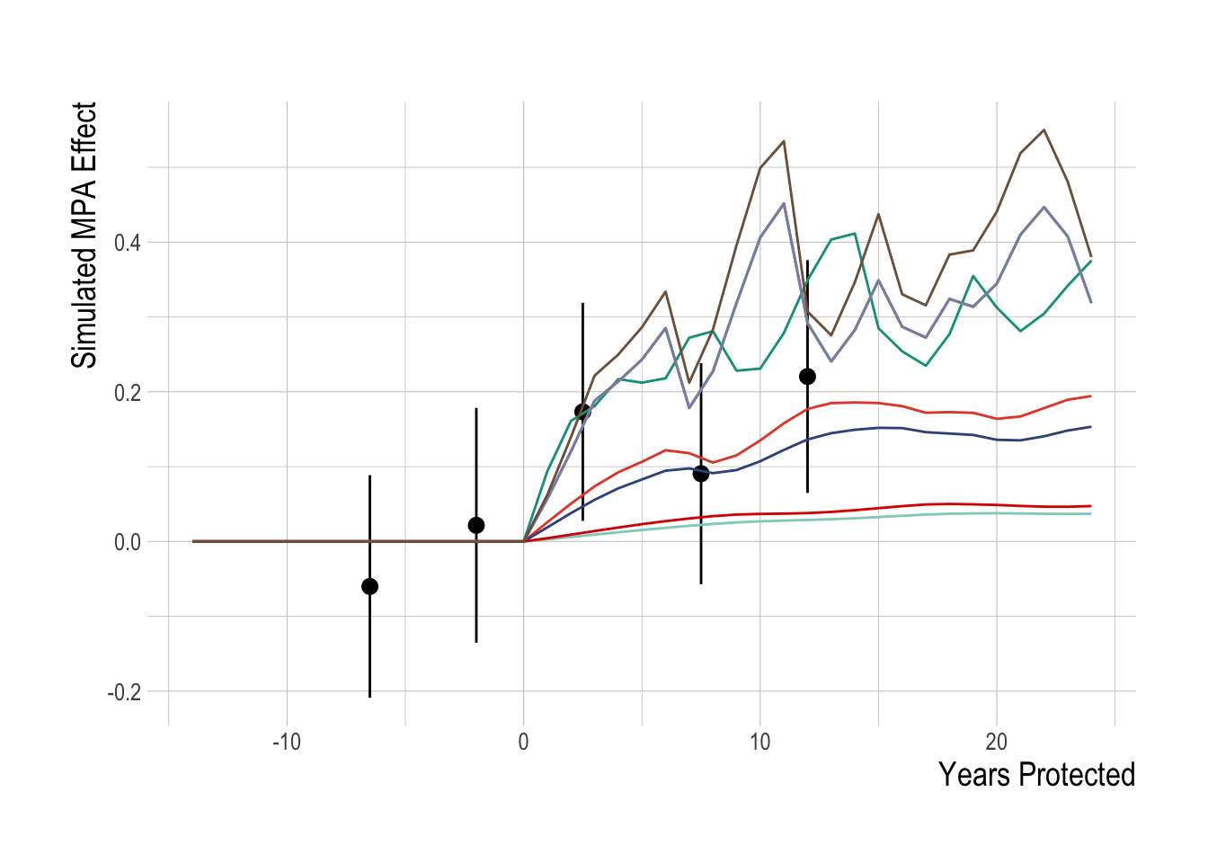
Figure 2.11: Simulation testing of identification strategy. Colored lines show true MPA effect for simulated targeted species. Black points represent mean estiamted regional MPA effect over 5-year blocks (range indicate 95% confidence interval)

Since we have evidence that our estimation model functions if its assumptions are satisfied, we then turned to estimating the regional MPA effect from the PISCO data. While individual species in the survey have their own abundance trends, the model assumes that abundance of targeted and non-targeted species each come from a common distribution. Assuming parallel pre-treatment trends, which visual (Fig.2.15) and statistical (Fig.2.16) assessment do not rule out, the trend in the underlying mean abundance index of non-targeted species post MPA serves as our control for unobserved environmental variables that could also affect the trends in the mean density of targeted species. So, by this logic, we should see no significant divergence between the targeted and non-targeted abundance trends pre “treatment” (implementation of the MPAs), and then some divergence between the treated group (targeted species) and the non-treated group (non-targeted) post treatment (if the treatment has an effect).

Under these idealized circumstances, the magnitude of this divergence between the treated (targeted) and non-treated (non-targeted) groups post treatment is an estimate of the causal effect of the treatment (the implementation of MPAs). It is important to consider what exactly this model controls for (and what it does not). Under the parallel trends assumption, we assume that both the targeted and non-targeted fishes respond the same way to non-modeled environmental drivers. For example, the Channel Islands region experienced a major El Niño event from 2014 to 2016. While we include variables such as deviations from each specie’s preferred thermal niche, along with kelp cover, in our model, these are clearly not the only factors affected by El Niño. However, if the parallel trends assumption is correct, the El Niño effects that are not explicitly included in the model are controlled for by the trend of the non-targeted fishes.

However, this clearly does not control for differences in responses to non-modeled variables between the treated and non-treated groups. For example, the model only pre-MPA data from 2000 through 2002. The parallel trends assumption appears plausible over that time period (Fig.2.16). But, this pre-treatment period does not include an El Niño, while the post-treatment period does. Therefore, while the parallel trends assumption looks plausible from the pre-treatment data, it is possible that targeted and non-targeted fishes respond in a systematically different manner to El Niño, therefore violating the parallel trends assumption and invalidating the “causal” interpretation of the model. Similarly, the model cannot account for additional shocks to the targeted species beyond the MPAs. For example, while we control for total landings of each targeted species in the Santa Barbara region, it is possible that within that region fishing effort became increasingly concentrated around the Islands, driving down local densities of fished species. The model cannot control for this unless the appropriate data are correctly incorporated into the model explicitly (and these data were not available at the time of this study).

The model also assumes that the targeted and non-targeted fishes do not directly or indirectly affect each other. This assumption is clearly violated on some level: all the fishes in this analysis are part of the same ecosystem and therefore interact to some degree. For example, if the protection of targeted predatory fishes results in increased mortality of non-targeted fishes, the model would attribute that as an increased regional effect (greater divergence between the abundance of targeted and non-targeted species). Given the time scale of analysis (15 years of protection), we do not feel that massive trophic cascades are likely to have developed yet, given both the pace and complexity of trophic cascade development (Babcock et al. 2010; Pershing et al. 2015). A complete assessment of evidence for trophic cascades in the Channel Islands is beyond the scope of this study, but to address this question somewhat we utilized convergent cross mapping sensu Sugihara et al. (2012) to test for a significant causal signal between different broad trophic groups in the data, implemented in the rEDM package in R.

Following methods laid out in Clark et al. (2015), we pool the abundance of each broad trophic group by region (Fig.2.12. This uses the data from the islands as “replicates”, requiring the assumption that the islands are all part of the same dynamic system, but allowing us to take advantage of the extra information provided by each island to further resolve the reconstructed manifolds. Using these aggregations, we then test whether the variables can be properly embedded, i.e., if they have predictable manifold dynamics. We do this through a simplex forecasting test, using an individual timeseries’ own lags to build a manifold. For each timeseries, the “best embedding dimension” is an approximation of the dimensionality of the dynamic system, in other words, the number of dimensions that define and predict the evolving states of the timeseries. This analysis shows that only the carnivore and herbivore groups show evidence of predictability within the timeseries (skill approaching zero within the tested embedding dimensions, Fig.2.13).

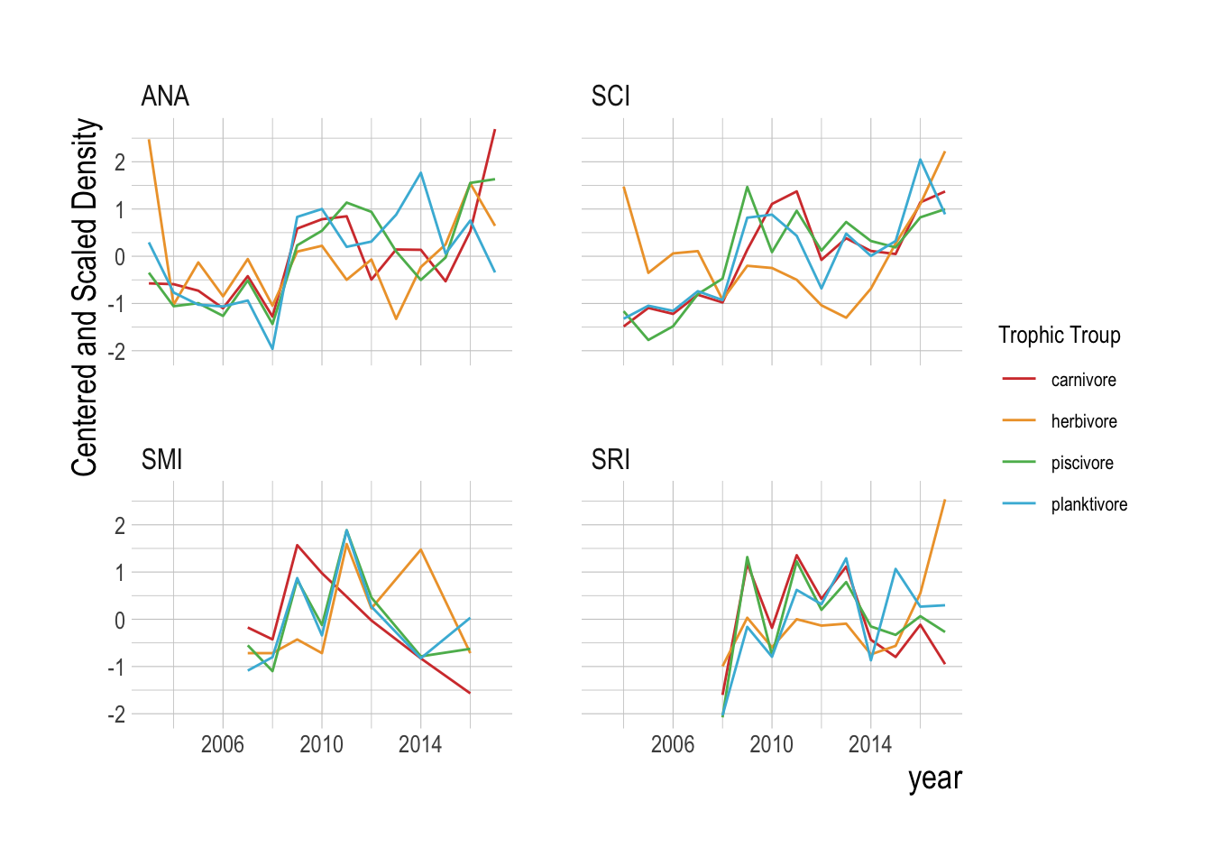
Figure 2.12: Centered and scaled densities by broad trophic group and island over time

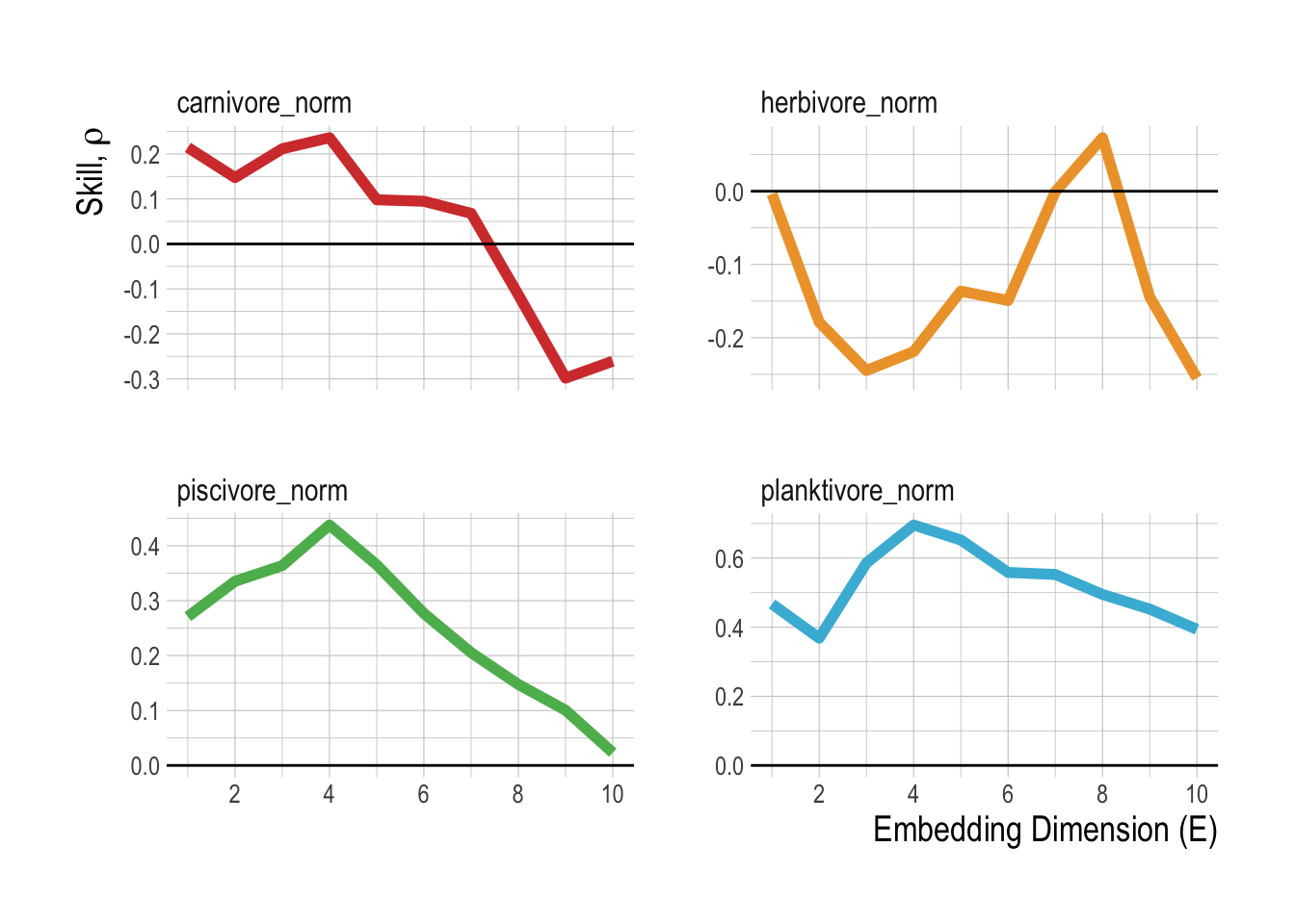
Figure 2.13: Predictive skill as a function of embedding dimensions

Focusing on just these two groups then, we can test for a causal relationship through Takens theorem using convergent cross mapping. Generalizations of Takens’ theorem indicate that if two variables (in our case, species or physical variables) are part of the same dynamic system, their individual dynamics should reflect their relative causal influence. In other words, if one variable is causally forced by another, that forcing should leave a signature on the first time series. Convergent cross mapping (CCM) tests for causation by using the attractor/manifold built from the time series of one variable to predict another (hence the “cross-mapping”). In simple terms, the causal effect of A on B is determined by how well B cross-maps A.

There are two criteria for CCM to establish causality: First, and most obviously, predictive cross-map skill using all available data should be significantly greater than zero. Second, that predictability should be convergent. Convergence means that cross-mapped estimates improve with library length (the number of state-space vectors used to build the attractor), because the attractor is more fully resolved and therefore estimation error should decline. Convergence is key to distinguishing causation from simple or spurious correlation. If two variables are spuriously correlated and not causally linked, CCM should fail to satisfy this second criterion. Based on these criteria, there is some slight evidence that herbivores may be driving carnivore densities, but no evidence that carnivores drive herbivores (Fig.2.14). This analysis provides evidence that trophic cascades are unlikely to be a significant driver of our results. It is important to note though that this analysis does not mean that trophic cascades could not evolve, rather that we do not detect them with these data at this time.

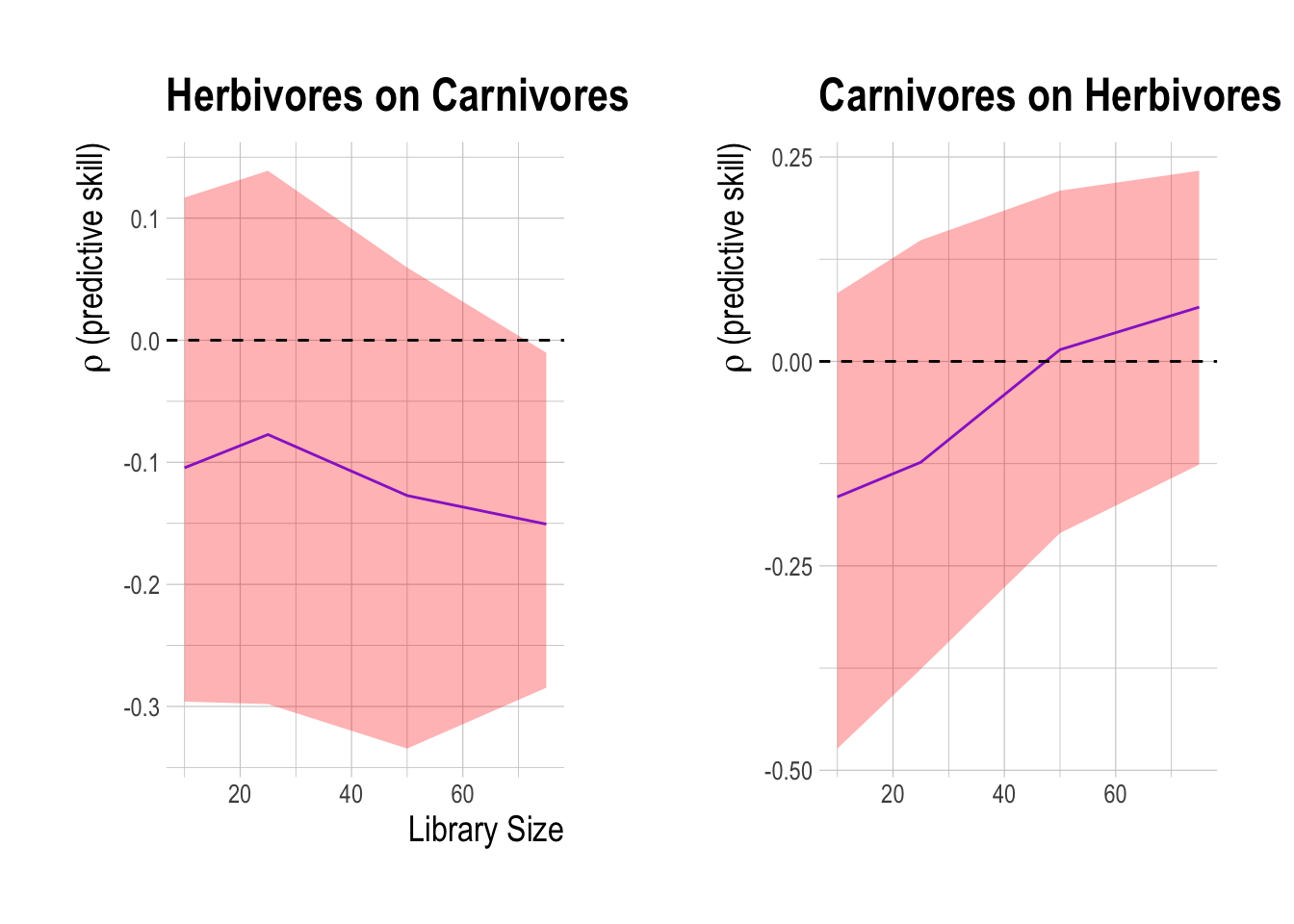
Figure 2.14: Cross mapping of effect of herbivores on carnivores (A) and carnivores on herbivores (B) in the PISCO data from 2000 to 2017. Shaded region show 95% confidence interval

The proposed identification strategy serves to control for some unobserved factors influencing densities of targeted and non-targeted species, but is unlikely to account for all of them. Before examining regression results, we can graphically examine the trends in mean densities for targeted and non-targeted species over time. We centered and scaled the mean annual densities for each species included in the analysis in order to compare the trends across species groups. Grouping the species by targeted and non-targeted status, we see evidence of pre-treatment parallel trends in the abundance indices, and of a divergence post MPA implementation. Beginning in around 2007 abundances of targeted species appear to start increasing faster than non-targeted species. However, from 2012 onward abundances of targeted species appear to be declining relative to the trend in the non-targeted species. Not controlling for any other factors that may affect fish abundances, the data suggests a possible increase in targeted species abundance (relative to the “control” trend of the non-targeted species) at first, followed by a decrease in the most recent years (Fig.2.15).

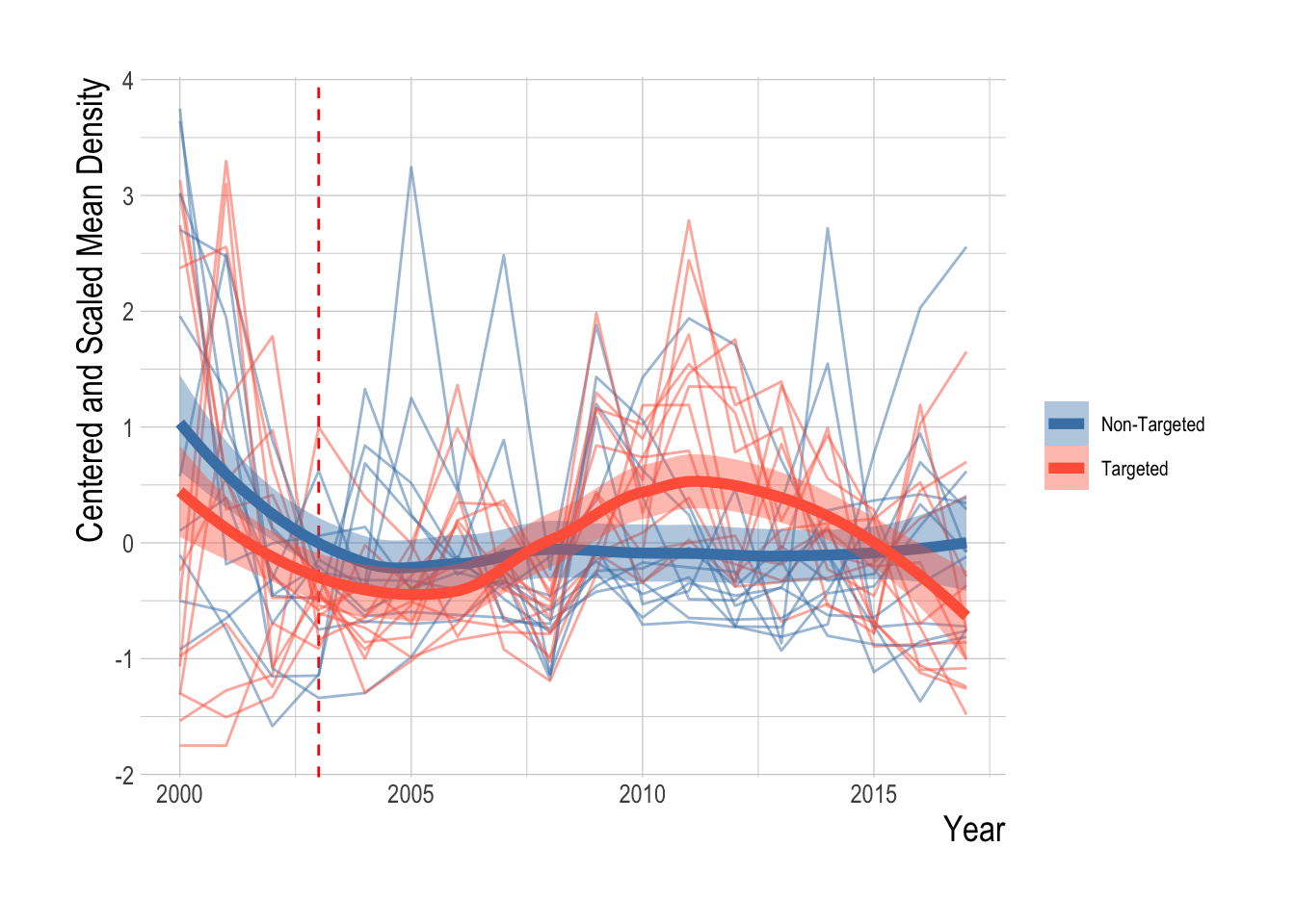
Figure 2.15: Centered and scaled mean annual density of included species (faded lines) and smoothed means of targeted and non-targeted groups (darker lines and ribbon representing 95% confidence interval of the mean) over time

We confronted these visual trends with our statistical analysis to estimate the divergence in the abundance trends of targeted and non-targeted fishes, controlling for factors such as observer effects, kelp and temperature, and unobserved environmental drivers through the parallel trends assumption. Using this analysis, we do not detect a significant change in the density of targeted fishes relative to the density of non-targeted fishes following the implementation of MPAs in the Channel Islands in 2003 (Fig.2.16). The mean estimated post MPA implementation divergence between the trends of targeted and non-targeted species was 0, indicating a roughly 0% divergence. However, it is important to note that just because we cannot a reject a hypothesis of zero divergence between the targeted and non-targeted groups does not mean that we have precisely estimated the effect size to be zero. Post implementation, the upper limit of the estimated 95% confidence intervals was 0.75 , and the lower limit was -0.79., suggesting the data have support for up to a 75% positive effect or a negative 75% effect.

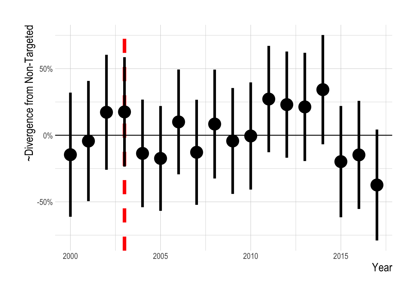
Figure 2.16: Estimated divergence in densities of targeted and non-targeted fishes throughout the Channel Islands (i.e. integrated across both inside and outside of MPAs). MPAs are implemented in 2003 (red dashsed line). Estimates are from a regression on log(abundance index), so estimated effects roughly correspond to percentage changes

As a robustness check to these results, we repeated our analysis utilizing data provided by the Kelp Forest Monitoring Program (KFM) conducted in the Channel Islands. Despite have similar but different methods and survey locations, we find almost identical estimated trends in divergences between targeted and non-targeted species using the KFM data (Fig.2.17).

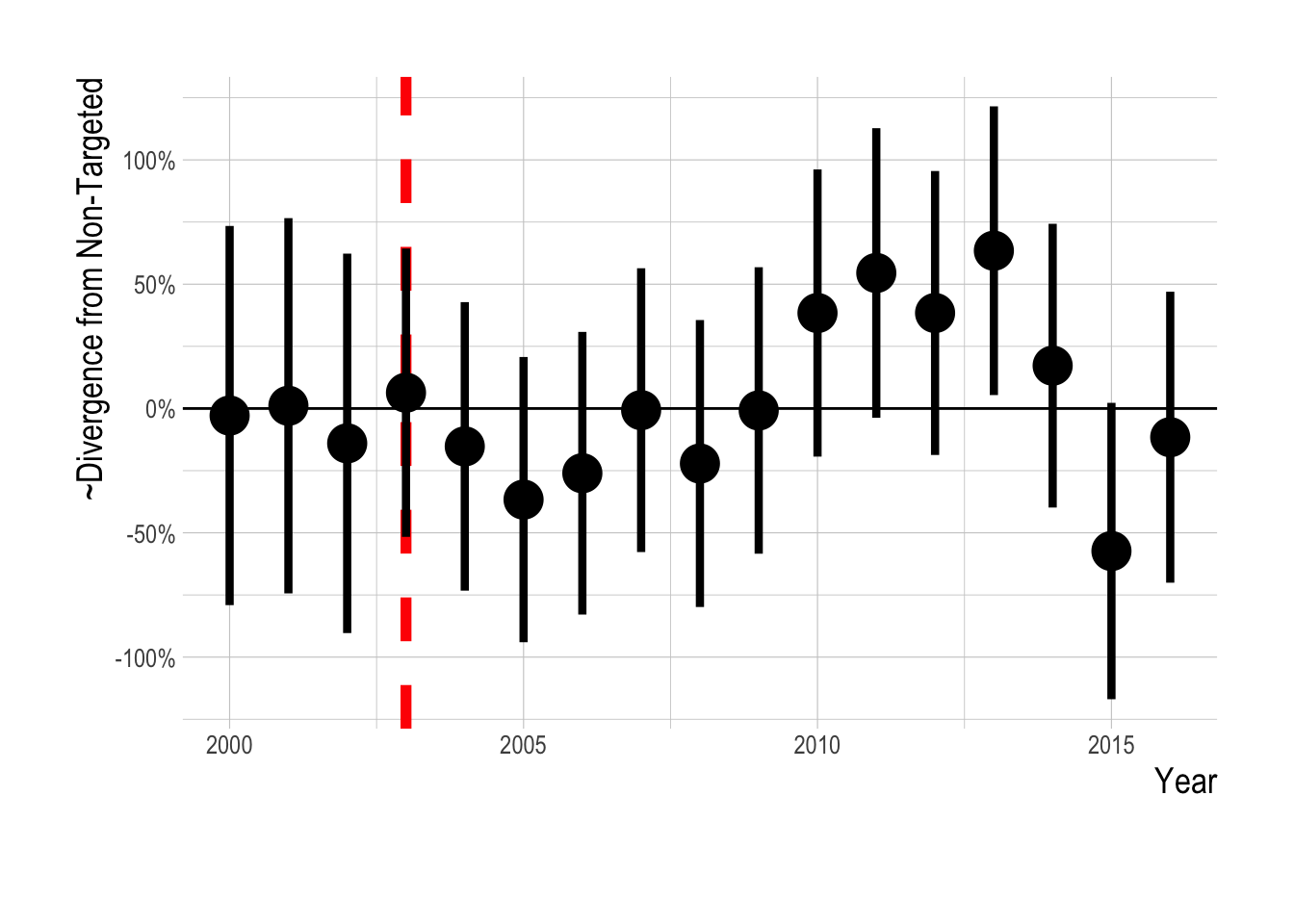
Figure 2.17: Estimated divergence in densities of targeted and non-targeted fishes in the Channel Islands (i.e. integrated across both inside and outside of MPAs) using the KFM data . MPAs are implemented in 2003 (red dashed line). Estimates are from a regression on log(abundance index), and so estimated effects roughly correspond to percentage changes

2.2.2.1 Regional Inside vs Outside MPA Effects

Given trends in mean densities observed in Fig.2.15, the “regional conservation effect” estimated by our model, defined as the divergence in trends between the targeted and non-targeted species across the Channel Islands region, is not surprising; By jumping through countless statistical hoops we reach a similar conclusion that we would just by looking at the divergences in the mean trends. The integration of data from inside and outside of MPAs is a possible explanation for this lack of a clear regional effect. If spillover is limited or has simply not developed yet, especially relative to the effect of fishing outside of MPAs, then it is possible that there is a clear positive effect inside the MPAs, a clear negative effect outside, and when we look across both types of sites we get an unclear average of the two.

To address this, we can first repeat some exploratory data analysis of trends in densities inside and outside the MPAs for targeted and non-targeted species. Caselle et al. (2015) provides a thorough look at this question of differences inside and outside of MPAs, we update the analysis here to account for our specific questions of trend divergence, potential differences in filtering methods, to include data up through 2017, and to utilize our estimation method on just the inside-MPA data. For all exploratory analyses, we consider the same top 23 consistently observed species. Looking first at simple trends in total mean biomass density across these species inside and outside of MPAs, we find evidence that biomass densities inside the MPAs is increasing faster (and is higher inside) than outside (Fig.2.18).

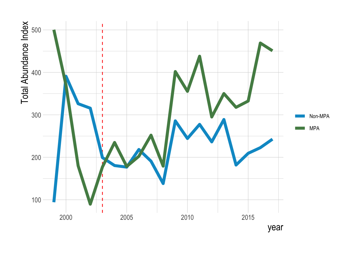
Figure 2.18: Mean aggregate biomass density (summed across all fishes) inside and outside of eventual MPA locations over time. Red dashed line indicates MPA implementation year

Our proposed identification strategy here though is not that total biomass density should be different inside and outside, but that the non-targeted species should serve as the control to the targeted. If we believe that the MPA effects are greater inside the MPA, then we would expect to see stronger divergences in biomass densities between these two targeted and non-targeted fishes inside the MPAs than outside

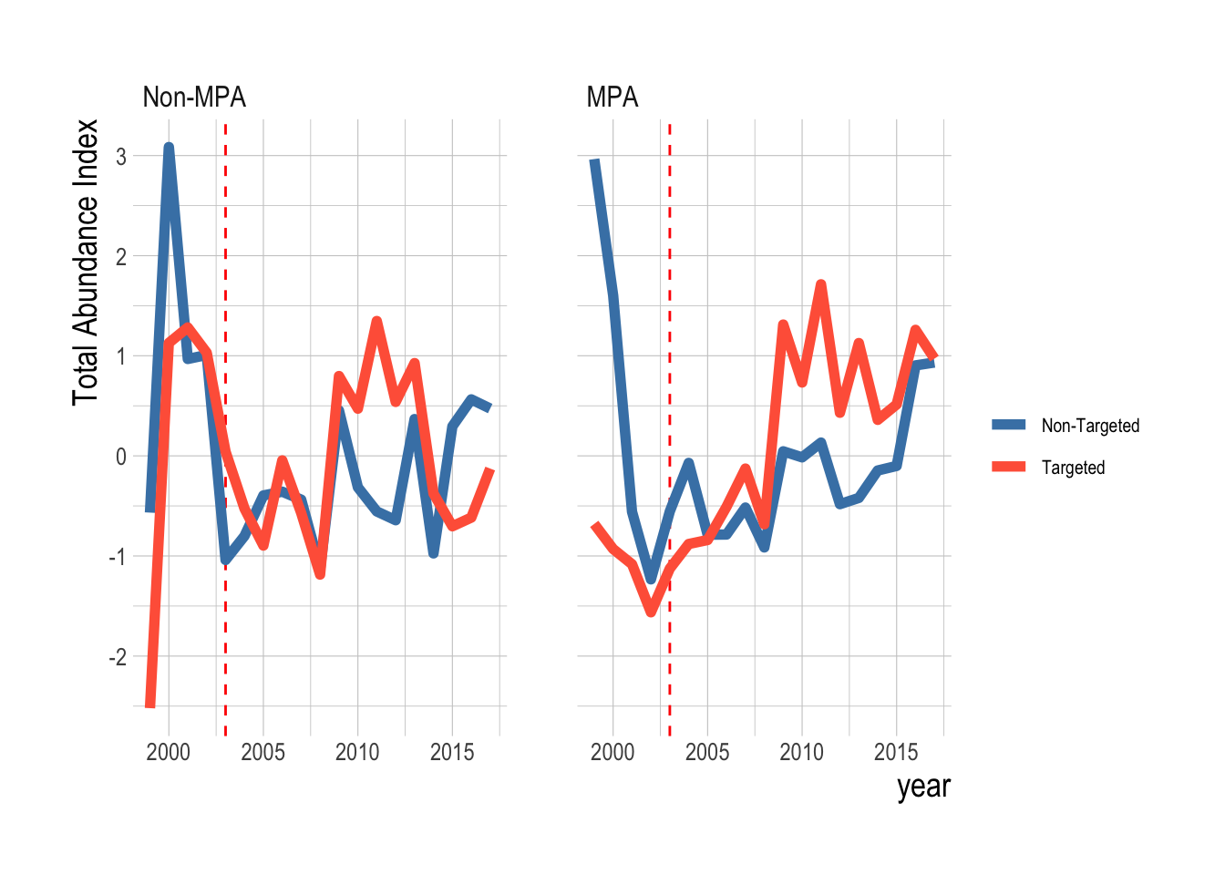
Figure 2.19: Trends in total biomass density inside and outside of eventual MPAs for targeted and non-targeted fishes. Red dashed line indicates MPA implementation year

Here we see a different picture. While there is some visual evidence that the targeted species were diverging from the non-targeted faster inside the MPAs than outside, both inside and outside we see that the trend in total biomass density of targeted species is trending downward, relative to the trend in the non-targeted species in recent years. This analysis is of total biomass density However, our model estimates the mean difference in targeted and non-targeted species. Both have their advantages, but we chose the mean to reflect a hypothesis that the MPAs would provide positive benefits across all targeted species. The total biomass density could be strongly affected by a sharp increase or decrease in one or two species, even if the mean trend is different. Examining the mean trends though, we see the same results (Fig.2.20).

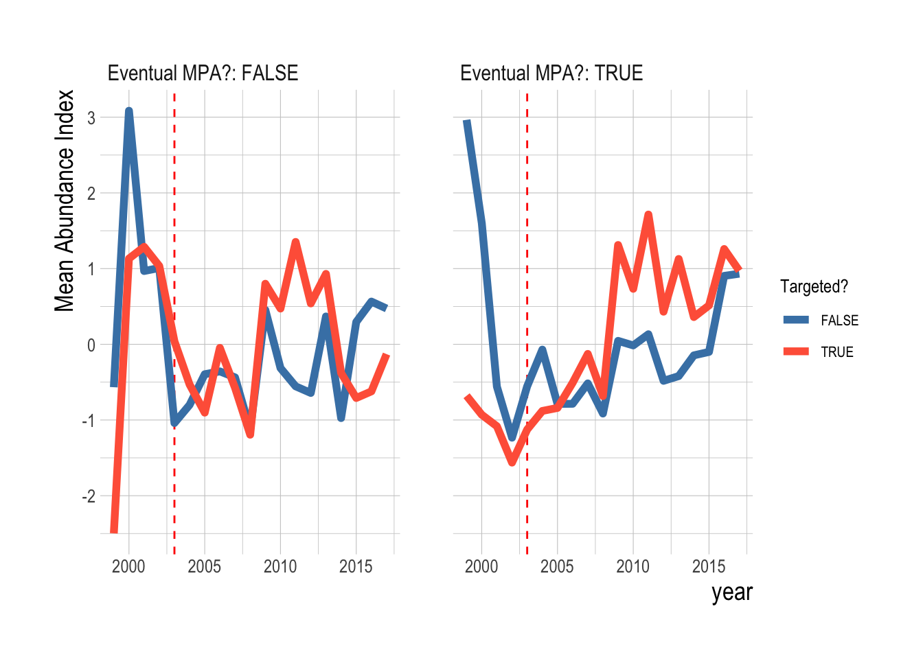
Figure 2.20: Trends in mean total biomass density inside and outside of eventual MPAs for targeted and non-targeted fishes. Red dashed line indicates MPA implementation year

Lastly, we can examine both the mean and individual trend to check clear species-by-species outliers in the overall biomass density trends. This analysis shows noise, but overall the targeted and non-targeted species seem to be following similar trends within their respective groups

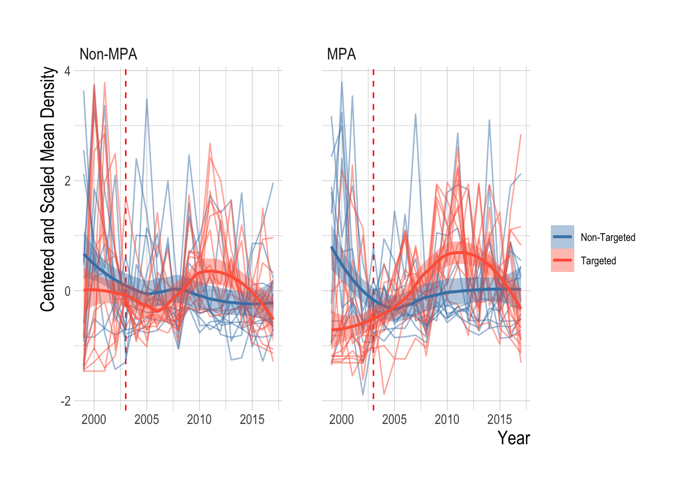
Figure 2.21: Centered and scaled biomass density trends for each fish grouped by targeted and non targeted (pale lines) and fitted LOESS smoother (with 95% confidence intervals around mean) and mean by targeted and non-targeted groups, inside and outside od MPAs. Red dashed line indicates MPA implementation year

These visual assessments suggest that similar to our results looking both inside and outside of MPAs, we would expect that our estimation model fitted only on data from inside eventual MPAs would reach similar conclusions as our results fitted to data from both inside and outside MPAs. To test this, we re-ran our analysis, but only using data from sites that are eventually placed inside MPAs. Our results reflect the same trends as displayed in the raw data and the statistical region-wide analysis, providing robust statistical support to the conclusions we would reach from visually examining the raw data (Fig. 2.22).

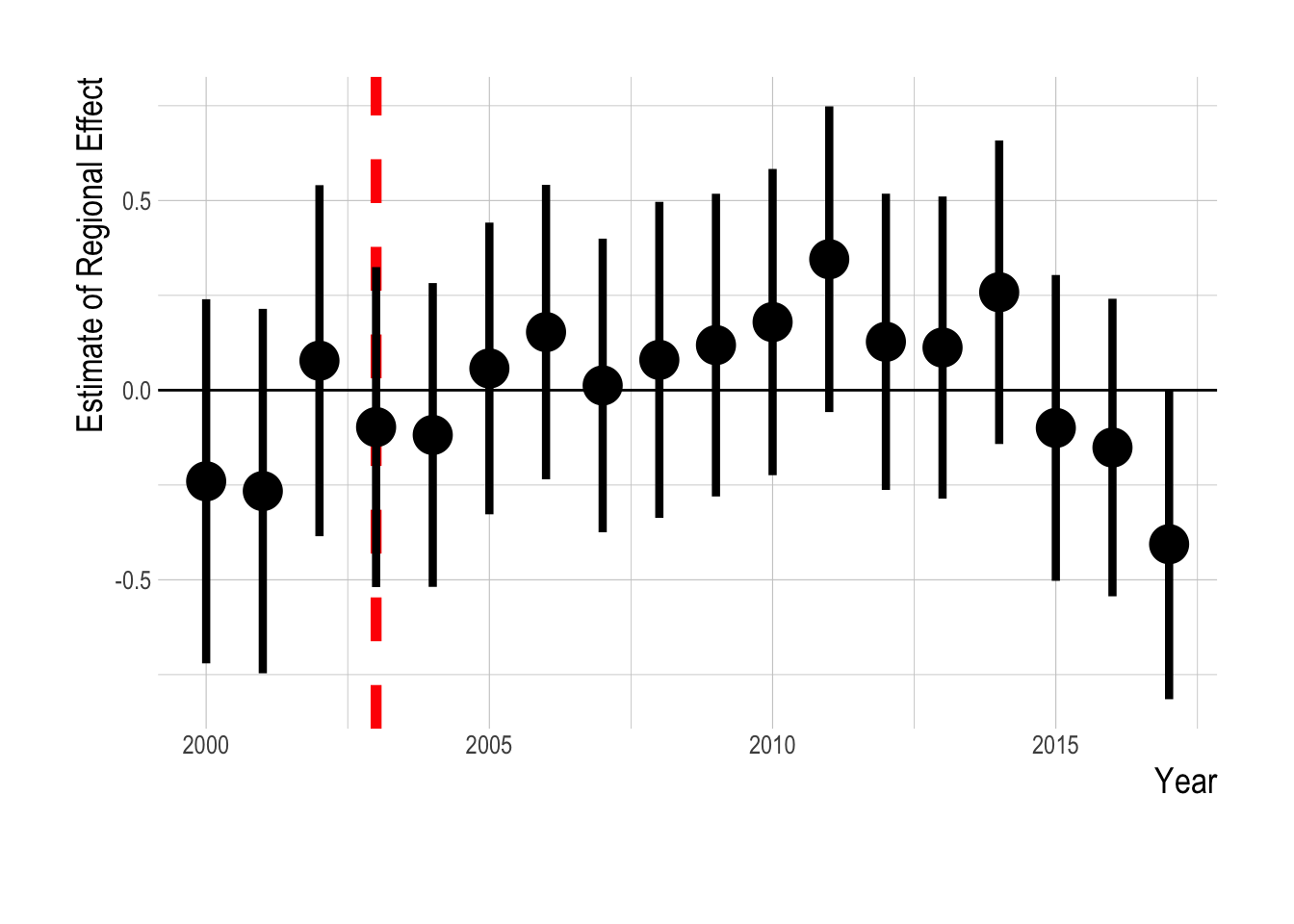
Figure 2.22: Estimated divergence in biomass densities of targeted and non-targeted fishes inside eventual Channel Islands MPAs. MPAs are implement in 2003 (red dashsed line). Estimates are from a regression on log(abundance index), and so estimated effects roughly correspond to percentage changes

2.2.3 Discussion

MPAs are playing a growing role in the management of marine resources around the world. While the primary purpose of MPAs is often to protect species and habitats within their borders, they are also looked to to provide spillover benefits to the ecosystems and fisheries surrounding them. The existence and magnitude of these spillover benefits has been a source of substantial debate for a some time, with the bulk of the conversation centered around qualitative or theoretical examinations of particular drivers of spillover (Hilborn and Walters 1992; Gaines et al. 2003, 2010; Gerber et al. 2003, 2005; Hastings and Botsford 2003; Hilborn et al. 2004a,b; Walters and Martell 2004; Botsford et al. 2008), or in detecting empirical evidence of the existence of spillover (Russ and Alcala 1996; e.g. Halpern et al. 2009), but not the net regional effects of MPAs. As many of the MPA networks around the world become mature enough for analysis, it is critical that we take a step to consider what evidence we can expect to observe, and what we have in fact seen in natural systems.

While a large body of literature has discussed the factors affecting the regional-scale conservation outcomes of MPAs, we know of no other study that has synthesized much of the key theoretical predictions of the literature into a comprehensive simulation framework to address the cumulative impact of these drivers on the regional effects of MPAs. Our results present several important insights for understanding what we might expect the effects of MPAs outside their borders to be. First, we see that incorporating a broad, but still limited, set of life history, MPA, and fishery characteristics produces a vast array of potential regional conservation effects, from actual net conservation losses (in cases for example of short-term constant-catch, moderate pre-MPA depletion, and smaller MPA sizes), to massive conservation and fishery gains (e.g large MPAs in a very depleted fishery). These wide ranges of outcomes persisted even in extreme cases; small effects were possible in very depleted fisheries, and larger effects were possible in cases of moderate depletion. One important result of this analysis is that looking across the range of “smaller” MPAs (covering 25% or less of the region), the median regional effect size was relatively small, both in percentage gains relative to the without-MPA scenario, and in percentage of unfished biomass recovered, up until the fishery was strongly depleted (Fig.2.4-2.6).

This has important implications for our ability to empirically detect these effects in natural systems. Marine environments are complex and noisy systems, subject to both large amounts of natural variation and measurement error. Our simulation results suggest then that it will be relatively difficult to detect the regional-scale effects of MPAs in many cases of smaller MPAs and moderately depleted fisheries; separating out say the median simulated population effect of a 0.0035711% of unfished biomass is a difficult task even in a carefully studied environment. With that in mind then, we should not be surprised that our analysis was unable to determine a clear regional divergence between the densities of targeted and non-targeted species throughout the Channel Islands in the 15 years since the newest set of MPAs were implemented in that region.

What can we infer about the regional effects of the Channel Island MPAs based on the available data and our analysis? At the simplest level, we cannot detect a significant divergence in densities of targeted and non-targeted fishes over the 15 years since the implementation of MPAs in the Channel Islands. However, it is important to note that we also cannot say that there has been no divergence. The 95% confidence intervals surrounding our year-to-year estimates of the divergences have a mean range of 1, and cross zero in nearly every year (indicating that both positive and negative divergences have support from the data). Since the regression model is a log-linear model (predicting log density indices), we can interpret the the “divergence” coefficients roughly as percentage differences in the densities of targeted and non-targeted. The upper end of of our estimated confidence intervals corresponds to a roughly 50% increase in densities of targeted species relative to non-targeted, while at the lower end a 50% decrease is possible. Within these ranges though, the mean effect size was 1%, which corresponds closely with the median MPA effects predicted by our simulation analysis for moderately exploited species protected by a reserve network covering ~25% of the region’s area.

Do these estimated divergences represent the regional effect of the MPAs? There are clear reasons why we might think not: differences in responses to environmental drivers such as El Niño between targeted and non-targeted species, as well as non-MPA related fishery changes, are both plausible and capable of distorting our results. Trophic interactions could also positively (if increases in targeted predators drive down densities of herbivorous non-targeted species for example) or negatively (if MPA mediated trophic cascades result in increases in both targeted and non-targeted densities) bias our results. However, while these concerns are important, they are not sufficient cause to dismiss our strategy for estimating the regional conservation effects of MPAs outright.

First, the assumptions of our identification strategy and operating models (e.g. no trophic interactions) reflect the underlying assumptions of much of the theoretical and simulation based literature on MPA effects used to motivate much of modern MPA design (Gaines et al. 2010; and fisheries management more broadly, Fulton et al. 2015). This of course does not mean that these assumptions are correct, but dismissing our results purely on the basis of for example the potential for trophic interactions requires then that we also rethink much of the work on which MPA design is based (we can’t use single species models to predict MPA effects but dismiss a single species model to estimate their effect). All else being equal, most standard models of MPA effects would predict faster and more substantial changes in densities of targeted fishes post MPA implementation than for non-targeted species, which is exactly what our model is designed to detect. If trophic feedbacks in the form of decreases in non-targeted prey as targeted predators rebound do exist, this would actually serve to positively bias our estimate of regional conservation MPA effects. Our cross-mapping analysis does not suggest that trophic interactions are playing a substantial role in our results.

Second, our identification strategy is an improvement over the alternatives that are likely to be available in most cases. We could simply compare regional densities of fish before and after MPA implementation. Doing so in the case of the Channel Islands suggests that, controlling for observable covariates, densities of targeted species have declined substantially post-MPA [Fig.2.35]. The reason we are skeptical of this conclusion though is of course that other non-MPA factors for which we do not have adequate data to include in the model could be driving that decline. The relatively parallel pre-MPA trends in densities of targeted and non-targeted species suggests that this is indeed the case. We would of course prefer some form of control group rather than simply before-after comparisons. However, for all but the most specialized of cases we are unlikely to ever have effective spatio-temporal controls for MPAs (e.g. an MPA-less carbon-copy of the Channel Islands, though see (???) for an example of using different regions as attempted controls). Given these constraints then, measuring the regional divergence in targeted and non-targeted species is likely to be among the best available options for empirically estimating the region-wide conservation effects of MPAs given the kinds of data that are often collected in conjunction with MPAs (transect surveys inside and outside of reserves).

Along with the identification strategy, there are clear fundamental challenges to accurately estimating densities of different species across a large marine region. Dive conditions can greatly impact the ability of divers to make accurate counts. Density estimates of highly mobile species can be positively biased [Ward-Paige2010]. Funding constraints limit the ability to consistently monitor all important sites throughout a region. This analysis also only considers finfish; invertebrate targeted species such as urchin and lobster that often have small home ranges in their adult stages may demonstrate clearer MPA effects (e.g. Kay et al. 2012).

One potential alternative to a regression-based identification strategy would be structural modeling of MPAs within a stock assessment process (Field et al. 2006). Conditional on having high quality data, the key problem in the regression based approach we present here is isolating MPA spillover effects, fleet responses, and environmental shocks from each other. Integrated stock assessments (as described in Hilborn and Walters 1992) provide a potential way to estimate these effects. The ability of larval spillover to provide conservation gains assumes a relationship between spawning stock biomass and recruitment. Therefore, within a stock assessment the relative importance of estimated recruitment deviates to estimated population trajectories could provide an index of how much increases in spawning stock biomass resulting from an MPA are contributing to recruitment vs the effect of environmental drivers. Similarly, spatial estimates of fishing mortality and biomass can help answer whether total mortality and biomass have gone up or down following MPA implementation. Such an analysis though would require integrating data from inside and outside of MPAs (which fishery dependent data cannot do) and research programs such as PISCO provide a natural platform for this type of analysis to build off of.

Our estimated regional divergences in the densities of targeted and non-targeted fishes present an imperfect but improved (relative to alternative options) window into the regional effects of the Channel Islands MPAs. Our results leverage the evidence of parallel trends between the targeted and non-targeted fishes to refute the conclusion of post-MPA declines in densities we would reach if we simply looked at pre-and-post MPA densities of targeted species. But, we also do not find clear evidence for substantial increases in densities of targeted species, relative to the trend we would expect given the densities of the non-targeted species. We do see some evidence for an increasing trend in targeted densities from 2003 to 2014, but this period is followed by signs of decreases from 2015 onward. The magnitude and direction of both of these changes are plausible effects of MPAs, according to our simulation analysis. The early upward trend could certainly be attributable to larval or adult spillover from the MPAs, as well as biomass buildup inside the MPAs themselves. The later decline could be due to concentrated fishing pressure outside the reserves.

It is also possible though that factors exogenous to the MPAs themselves are driving the apparent recent decline in the trends of targeted species relative to the non-targeted. For example, an increase in fishing effort resulting from market forces could explain the recent downturn, but we would not want to attribute that as a regional conservation effect of the MPAs themselves (though including estimates of commercial landings for species in our analysis did not change our results, suggesting that this downtown cannot be explained by total catch alone). The presence of a downward trend in the estimated regional when we look just inside the MPAs suggests that environmental drivers may be the culprit here. If we assume that the MPAs are indeed well enforced and large enough to provide some substantial protection from fishing for at least some of the targeted species, which we have every reason to believe (Caselle et al. 2015), then if the cause of the recent downturn estimated by our model were increased fishing, we would expect to see that effect masked or at least dampened in the within-MPA data and analysis. That we still see the decline in the within-MPA data provides evidence that a broader environmental event is depressing the trend in the targeted species, such as the large El Niño events of 2009-10 and 2014-2016. This is supported by the clear warming signal in measured sea surface temperatures throughout the Channel Islands in recent years (Fig.2.23). While our simulation analysis focused on the structural characteristics of a fishery system that could make it more or less able to provide regional scale conservation benefits, these results highlight the critical importance of environmental drivers in the actual year-to-year effects of marine conservation policy.

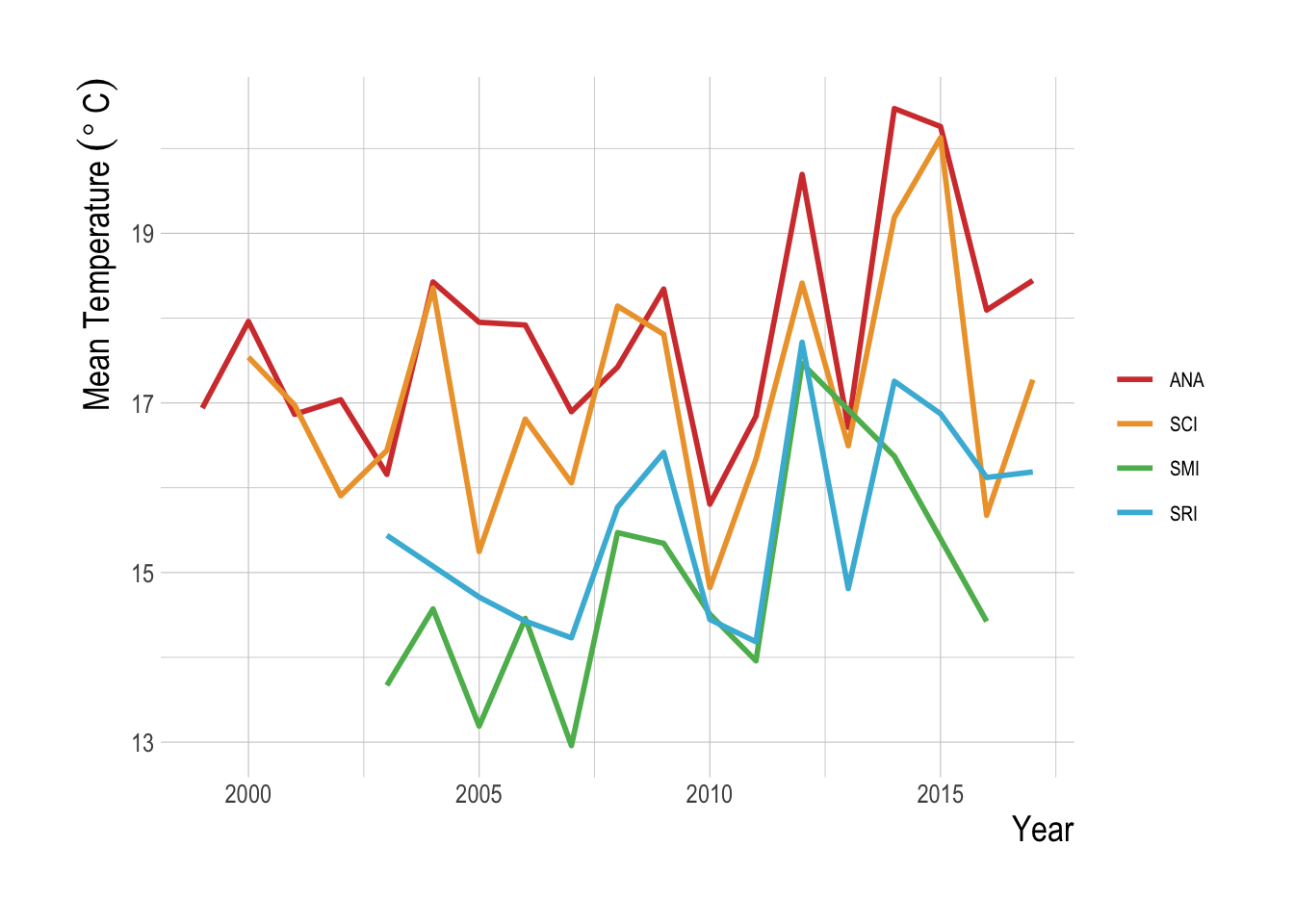
Figure 2.23: Mean temperature over time at each of the Channel Islands included in this study

Despite the vast amount of rigorous data collection before and after, our identification strategy was unable to identify a clear signal of the effect of MPAs on the regional densities of targeted species. Our simulation analysis indicates though that we should not be surprised by this. The Channel Islands MPAs cover approximately 21% of the waters in the Channel Islands, and while formal stock assessments are not available for many of the targeted species in our analysis what evidence we have does not suggest they as a group they are heavily overfished. Our simulation analysis would suggest then that the percentage difference in densities of targeted species with and without MPAs should be on the smaller end (10% or less), and therefore be challenging to detect given the natural variation of marine ecosystems and the error inherent in visual survey programs such as those the PISCO data used here. What then does this suggest for the design and monitoring of MPAs?

Real world-policy making is inherently an exercise in utilizing best available theory, experience, and modeling to make decisions that are often difficult or practically impossible to empirically test. Despite our best efforts we are unlikely to ever truly “know” the effect of our efforts to mitigate climate change, but must instead rely on comparisons to best available modeling outcomes to understand how effective our policies have been. Similarly, given the complexities of marine systems much of our decisions on MPA design will have to be based on effective modeling. While we are hardly the first to point out that bio-economic models are a critical tool for MPA design, our results help indicate a minimum floor of model complexity to provide candid assessments of regional MPA effects. While factors such as MPA size and degree of depletion are especially strong drivers, for all but the most extreme cases of each a wide array of effects, from negative to highly positive, are possible based on the complex interaction of factors such as fleet dynamics, movement rates, and recruitment timing. Confronting these interactions by considering the likely parameter space for a given region is a critical step then in understanding what likely regional effects of MPAs are. While models such as ours do require large numbers of parameters that may be challenging to obtain, our results show that working with communities to confront these uncertainties is preferable to sweeping them under the rug in favor of simpler models that are easier to parameterize but miss details that our results show can have dramatic effect on expected outcomes. Modeling effort such as this can then provide stakeholders with some idea of the range of regional effect sizes that might be expected for a given MPA network design, and in doing so design monitoring programs targeted at the species and fleets that modeling suggests may provide the clearest indication of MPA mediated effects. For cases where bio-economic modeling suggests small potential for MPA driven regional density effects, monitoring efforts can be targeted around detecting potential negative effects should they arise, i.e. evidence that the model is wrong, rather than exerting massive amounts of effort on what theory and modeling suggest may be a small effect size.

We focus mostly on regional conservation gains in this paper. However, fisheries spillover is often another important factor to consider (i.e. are fisheries better off with the MPAs than they would have been without them). The fishery benefits of MPAs are just as (and likely more) intensely debated than the regional conservation outcomes (Roberts et al. 2001; Hilborn et al. 2004b; Hilborn 2018; Sala and Giakoumi 2018). We only address fisheries affects briefly in this study, but our results highlight important tradeoffs and synergies between conservation and fishery spillover effects of MPAs. The good news from a fisheries perspective is also fairly obvious: Both the regional conservation and fishery benefits are expected to be greatest when the fished population is in an extremely depleted state pre-MPA, even over a 15 year time horizon, even for larger MPAs (though further work is needed to compare MPAs to alternative fisheries management strategies in these cases). For cases where a valuable and formerly abundant species is overfished, a large MPA may then provide large conservation and fishery gains for that species, while potentially having smaller impacts on other less depleted species. Our simulation results also do identify though a large parameter space where MPAs create tradeoffs between moderate conservation gains and moderate fishing losses. This type of projection analysis can help managers consider where in this space they may be. The most critical point with regards to conservation and fishery effects from our simulation analysis is that the conservation or fishery effects of MPAs cannot be reliably estimated without some knowledge and consideration of the dynamics of the fishing fleet outside the MPAs: over the short-term open access vs constant catch dynamics can make the difference between a substantial conservation and fisheries win to a more depleted stock with more expensive fishing.

MPAs are an important part of the marine resource management toolbox. Under ideal circumstances they can protect both individual species and ecosystem linkages, safeguard crucial habitat, and support local economies through tourism and fishing opportunities. However, our results show that the regional conservation and fishery benefits we should expect from MPAs are highly variable, and while we cannot assign probabilities to our simulated states of nature, we find that there are more opportunities for smaller effect sizes than large, especially in the short-term. Most importantly, our results highlight the critical importance of explicitly modeling the links between the biological effects of MPAs and the ways that humans respond to them. Large-scale empirical evidence supports our results that accurately predicting the effects of MPAs depends on understanding the human context in which they find themselves (Cinner et al. 2018). While this is far from the first effort at simulating MPAs, our model fills an important niche between more focused theoretical models that address a few drivers of MPA performance at a time but do not address complicated linkages between drivers, and more site-specific models that provide best available local results but are challenging to scale to different systems. This intermediate complexity model allows us to simulate tens of thousands of fisheries containing most of the key drivers of MPA performance identified by theory.

This process provides a unique survey of the likely regional effects of MPAs to fisheries and conservation, and places our empirical assessment of the regional effects of the Channel Islands MPAs in context. The Channel Islands are an intensely studied system, and the challenge of identifying a clear regional effect of the network of MPAs placed there in 2003 may seem surprising. However, our results show that in fact a smaller effect size, from the perspective of regional conservation gains, is to be expected in this system, and therefore the true effect will be very challenging to separate from environmental noise. The solution then though is not to give up on detecting effects, but rather to shift focus from identifying a specific effect size and instead use simulation analysis to appropriately set expectations for conservation and fishing stakeholders, and design monitoring programs around the species and situations that serve as effective indicators of the ability of an MPA network to achieve its objectives.

2.3 Methods

2.3.1 Simulation Model

The simulation model used in this analysis is roughly the same as the one described in Ovando et al. (2016). It is an age structured, spatially explicit, bio-economic model. Recruitment is assumed to have Beverton-Holt dynamics on average, though auto-correlated log-normal recruitment deviates can be specified. The timing of density dependence can be one of five forms presented in Babcock and MacCall (2011), ranging from independent density dependence in each patch to density dependence in a shared larval stage across patches. The model allows for both adult and larval movement, where larval movement is assumed to follow a Gaussian dispersal kernel based on the distance of each patch to the source patch. Adult movement is also modeled using a Gaussian dispersal kernel, but with the added option of density dependent movement as well. In the adult density dependent movement scenario we calculate the density gradient between each patch and every other patch, where the density gradient is calculated as

\[g_{i,j} = \frac{b_i}{b_i^0} - \frac{b_j}{b_j^0} + 1\]

Where i is the source patch and j is a sink patch, and \(b^0\) is the unfished biomass in a given patch. The density gradient \(g_{i,j}\) is used as a multiplicative modifier for the distance-based Gaussian dispersal kernel d, so that the net movement m of individuals from patch i to patches 1:J is

\[m_{i,j} = \frac{d_{i,j}g_{i,j}}{\sum_{1:J}d_{i,j}g_{i,j}} \]

Fishing activity is controlled by a fleet model that can take one of four forms: constant catch, constant effort, and open-access. For the constant effort and constant catch scenarios, a specified effort or catch level is set to achieve a target level of pre-MPA depletion, and that effort or catch is held constant post-MPA. For the open-access scenario, we model effort through a profit-response function, where profits are calculated per

\[profits_{t} \sim p_{t}q_{t}E_{t}B^{c}_{t} - c_{t}E_{t}^{\beta}\]

And then effort is modeled as

\[effort_{t} = effort_{t-1} + effort_{msy}(\theta\frac{profits_{t-1}}{profits_{msy}})\]

The operating model allows for time-varying and auto-correlated deviations in prices p, cost c, and catchability q. For all fleet model scenarios, effort is distributed in space in one of two manners: divided equally among all fish-able patches, and distributed in proportion to historic profits in each patch.

MPAs are implemented in the operating model by setting a specified percentage of the patches to be placed in a no-take MPA. Patches are then assigned to an MPA either in a linear fashion (left to right) or assigned at random throughout the patches. In all scenarios MPAs are implemented halfway through the simulated time series (allowing the pre-MPA fishing mortality to deplete the population to a desired level beforehand).

Using this operating model, we simulated MPA effects across 20,000 fisheries, where the regional effect is modeled by running the exact same fishery simulation with and without MPAs, and then calculating the difference in biomass in each year between the two scenarios (setting identical seeds for each simulation). The range of evaluated scenarios is presented in Fig.2.24 and Fig.2.25.

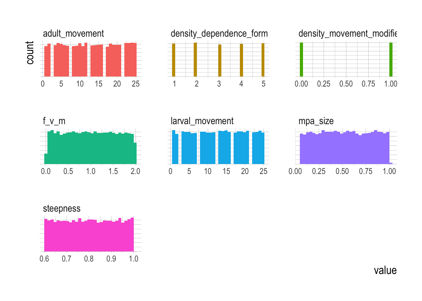
Figure 2.24: Histrogram of continuos variable levels across simulated fisheries

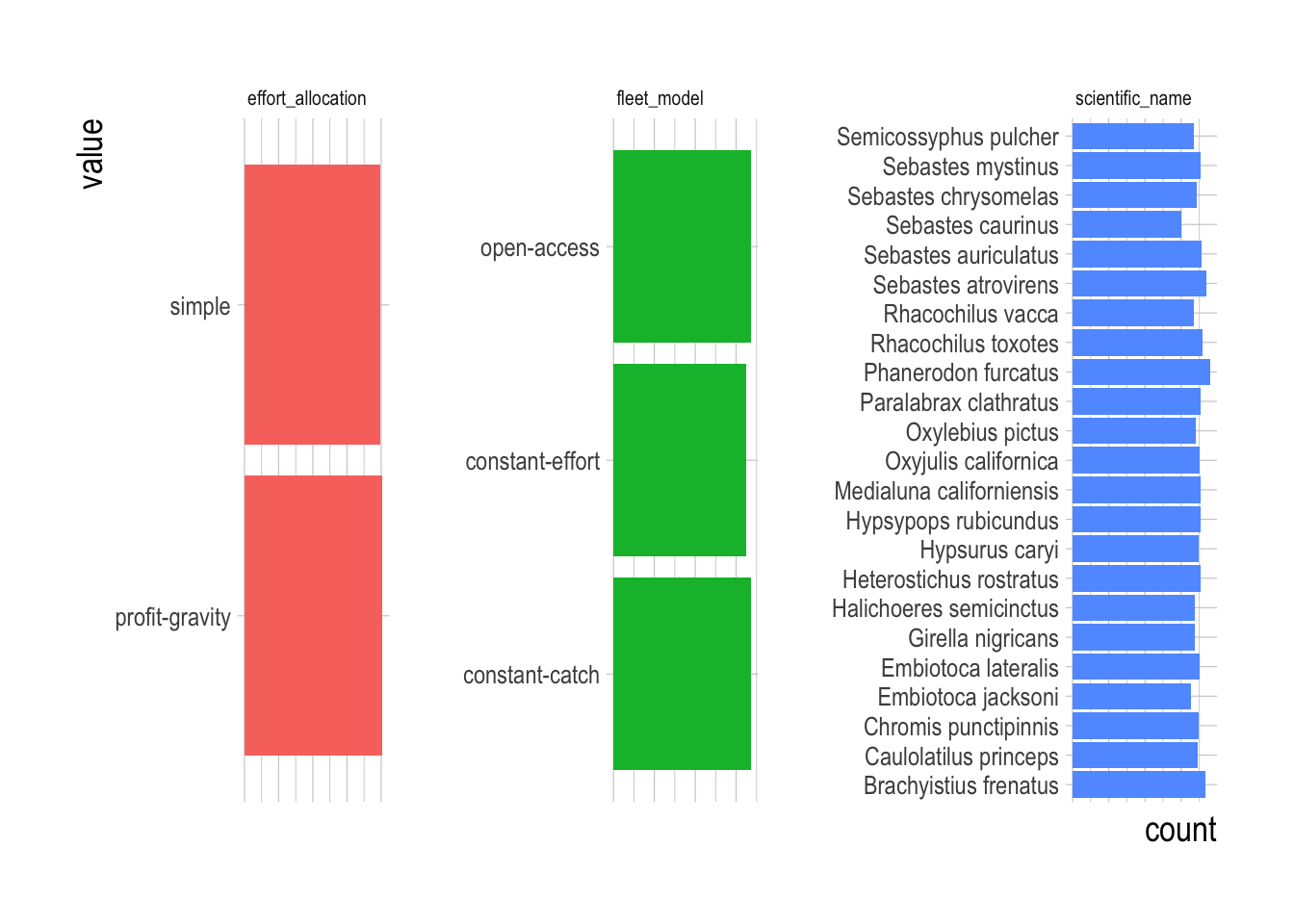
Figure 2.25: Counts of categorical variable levels across simulated fisheries

2.3.2 Regression Analysis

The regression analysis uses a mixed-effects hierarchical model. The raw data are estimated length compositions by fish species along a transect at a site. Lengths are converted to biomass per allometric relationships supplied by PISCO and supplemented by the FishLife (Thorson et al. 2017) package in R where needed. We performed some minimal data filtering to reduce noise in the data. We only include species that were observed at least twice in each year of the dataset (2000-2017) somewhere in the core Channel Islands (Anacapa, Santa Cruz, Santa Rosa, San Miguel). While some data are available from 1999, per consultation with PISCO we omit those data due to changes in survey protocols. We assign species to targeted and non-targeted groups per the PISCO classifications. This filtering process results in 11 non-targeted species and 12 targeted species remaining in the analysis.

The first stage of the regression is a log-normal delta model. The model estimates two regressions, the first is a binomial generalized linear model (GLM) with a logit link estimating the probability of observing a given fish species at a observation i (transect at time t). The probability that a given species was observed o at a given observation is distributed

\[o_{s,i} \sim binomial(\frac{1}{1 +e^{-\beta^{o}{X}}}) \] where \(\beta^{o}\) are the estimated coefficients for the observation model and X is a matrix of covariates that include random effects for each year in the data (2000 to 2017).

The expected density d of positive observations is modeled per a log-normal distribution

\[log(d_{s,i}) \sim normal(\beta^{d}X, \sigma_s)\]

where \(\beta^{d}\) are the estimated coefficients for the expected density model and X is the same matrix of covariates as used in the observation portion of the model and \(\sigma_s\) allows for each species s to have different standard deviations.

Our covariate matrix X contains both fixed and random effects. Fixed effects include the depth level of the transect, the sampling site, the month of the observation, the estimated surge at the transect, visibility, the depth of the transect, and the experience (and experience squared) of the diver conducting the transect. We classify each species into one of two clusters based on the mean longitude the species was encountered at, breaking the species into two groups: those primarily found in the western end of the Channel Islands those found more in the eastern end. We then estimate random effects for each island for each cluster

\[\beta_{island,cluster} \sim normal(0,\sigma_{cluster})\]

This allows the mean effect of each island to differ for each cluster, e.g. allowing the San Miguel, the eastern most island, to have a higher mean density for eastern species than for more western species (if the data suggest it).

The second critical component of the covariate matrix X are random effects for each year for each species

\[\beta_{year,species} \sim normal(0,\sigma_{species})\]

These \(\beta_{year,species}\) represent our “standardized” estimate of observed abundance of each species in each time step, controlling for the included covariates.

However, we still need to account for changes in the probability of detection over time. For that, we create a standard matrix of with rows equal to the number of years and columns corresponding to each of the columns in X, holding everything fixed at mean (or most frequently observed level for factors) levels for all variables in X except for the year and species interaction indices. Calling this standardized matrix \(X^{standard}\), the probability of observing a given species in year y is then

\[p_{s,y} = (\frac{1}{1 +e^{-\beta^{o}{X^{standard}}}})\]

In the same manner as described by Punt et al. (2000), The standardized index of abundance for species s in year y then is

\[I_{species,year} = p_{species,year}e^{\beta_{species,year}}\]

The next phase of the model requires us to estimate the mean abundance of targeted and non-targeted species over time. The concept here is that each \(I_{species,year}\) can be modeled by a regression that contains random effects for each year for targeted and non-targeted fishes, the assumption then being that there is a mean density for targeted and non-target species, and \(I_{species,year}\) represent deviations from that mean.

\[log(I_{species,year}) \sim normal(\beta^{effect}X^{effect}, \sigma_I)\]

\(X^{effect}\) contains both fixed and random effects. The fixed effects include an intercept and the temperature deviation for a given species in a year, where temperature deviation is

\[t_{s,y} = (t^{pref}_{s} - \bar{t_{y}})^2\]

where \(t^{pref}\) is the preferred temperature for species s (drawn form FishLife, Thorson et al. (2017)), and \(\bar{t_{y}}\) is the mean temperature encountered by that species in year y. We also include as variables in the model the mean kelp cover experienced by a given species in a given year, as well as the total fishery catches reported in the previous year for that species in the Santa Barbara region [drawn from the California Department of Fish and Wildlife database]. We also include random intercepts for each species in \(X^{effect}\). The most important random effects are year effects for targeted and non-targeted species

\[\beta_{year,targeted} \sim normal(0,\sigma_{targeted})\]

\(\beta_{year,targeted}\) is the mean log density of targeted species in year y, controlling for included covariates. Therefore, the final step in the model, the divergence in the standardized abundance trends of targeted and non-targeted species is

\[divergence_{year} = \beta_{year,targeted = 1} - \beta_{year,targeted = 0}\]

The model is fit in TMB to integrate the uncertainty across all levels of the model, with standard errors for each coefficient in the model estimated through the Laplace approximation.

Figures 2.26:2.28 present estimated effects for covariates included in the model, along with the raw estimated mean trends of the targeted and non-targeted species (while the difference between these trends is presented in our main results Fig.2.16).

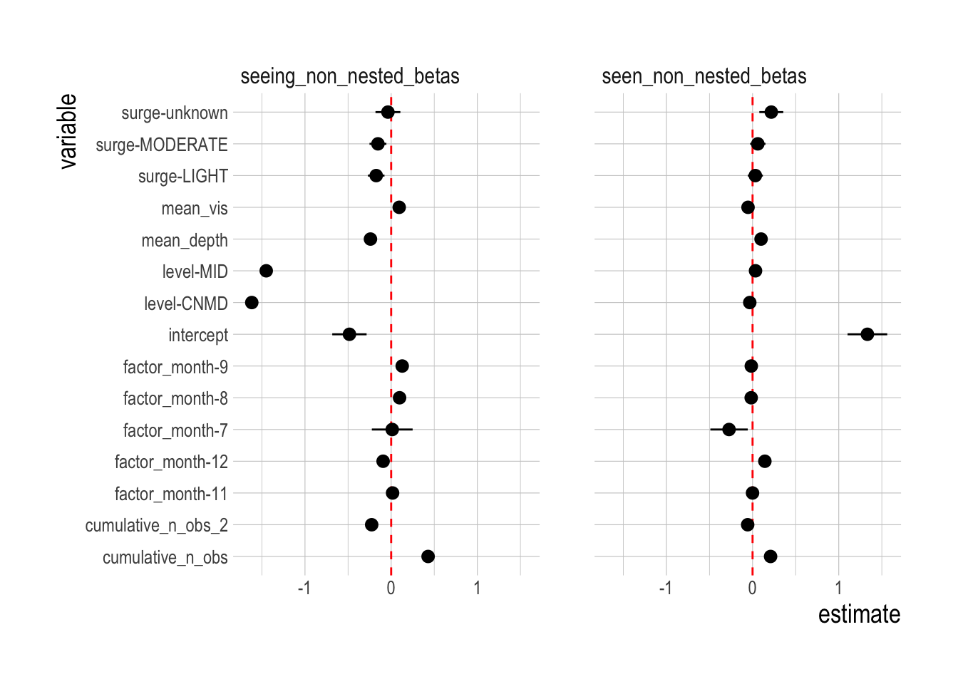
Figure 2.26: Estimated coefficients for non-spatial fixed effects in observation model (seeing) and observed model (seen)

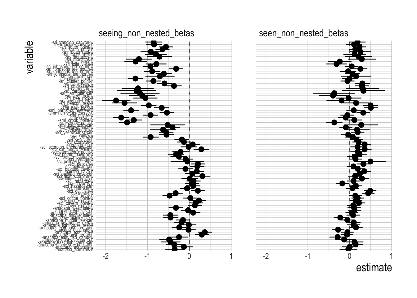
Figure 2.27: Estimated coefficients for spatial random effects in observation model (seeing) and observed model (seen)

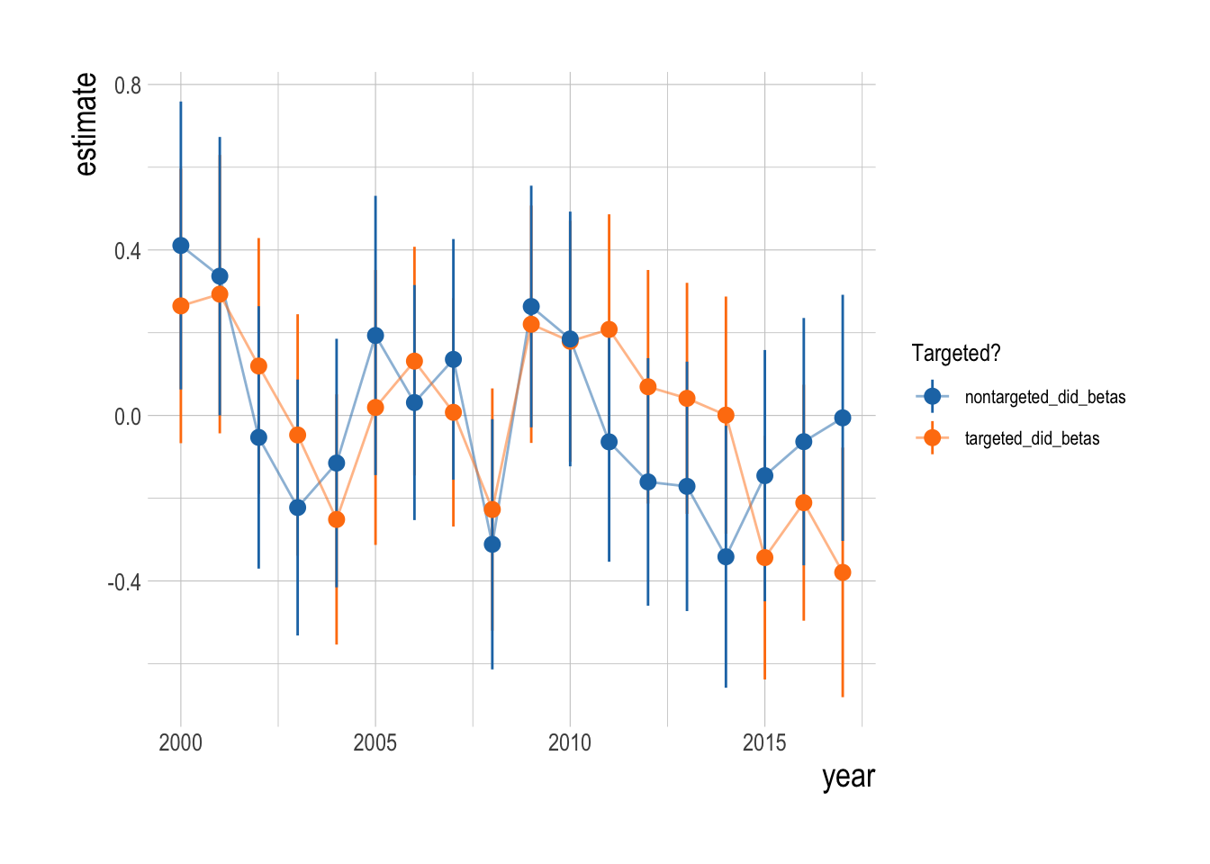
Figure 2.28: Trends in standardized mean abundance of targeted and non-targeted species

2.4 Supplementary Materials

2.4.1 Regression Diagnostics

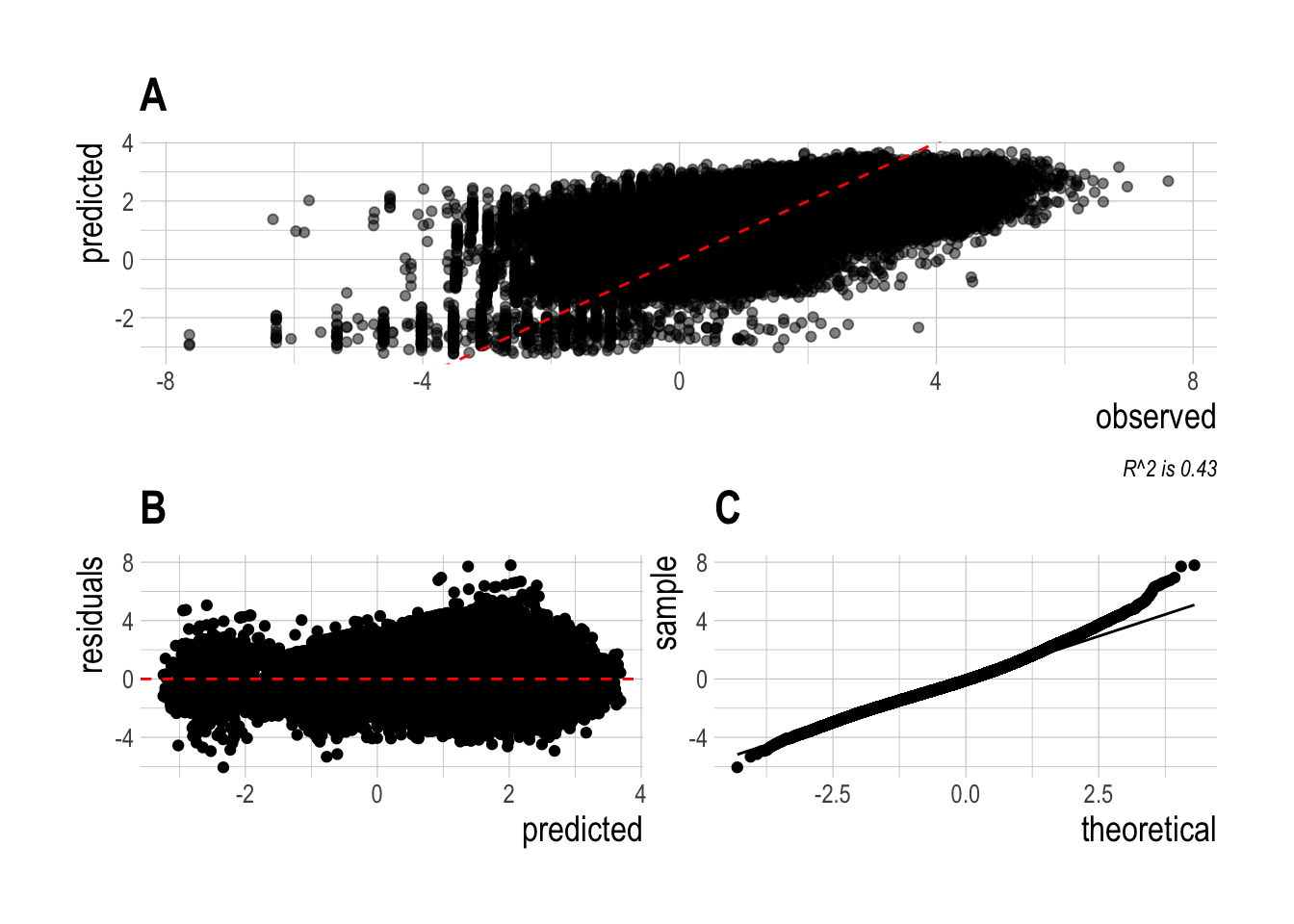
Figure 2.29: High level diagnostics for observed compontent of Delta-GLM: Observed vs predicted log densities (A), predicted log density vs residuals (B), and a normal qq-plot of the residuals (C)

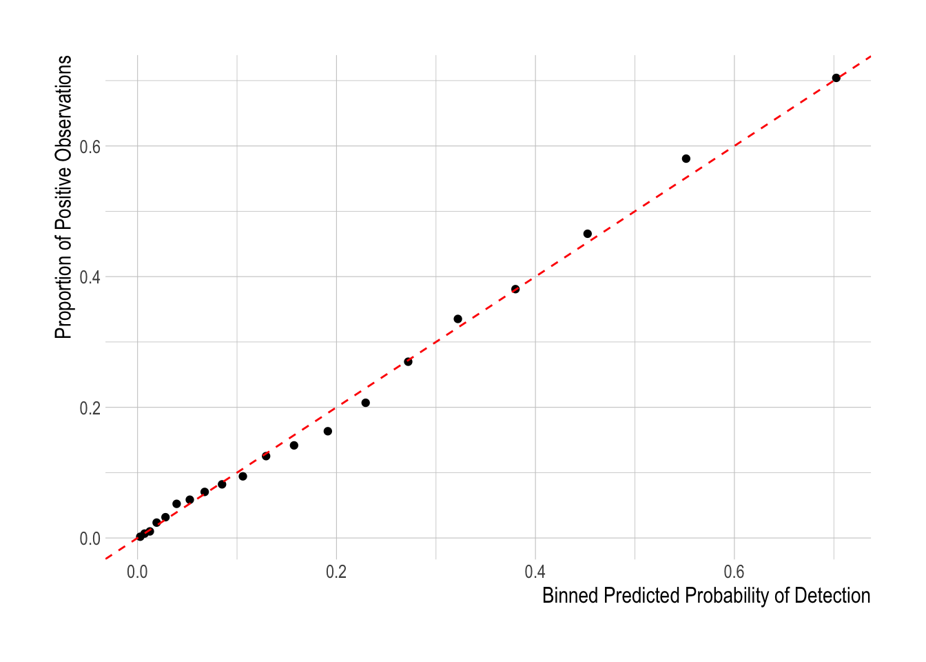
Figure 2.30: Binned mean predicted probability of detection provided by the first stage of the hurdel model vs observed proportion of positive detections

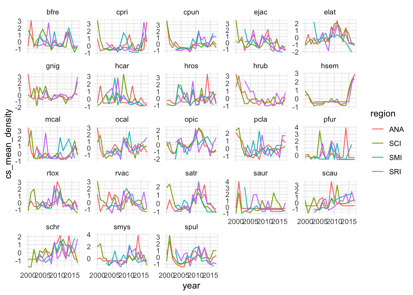
Figure 2.31: Mean density by island by year for each fish species included in the analysis

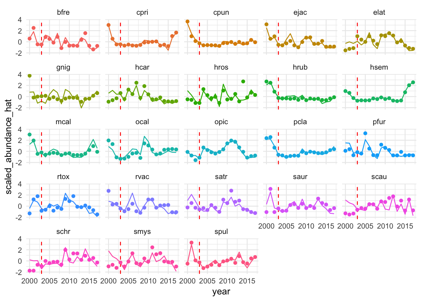
Figure 2.32: Raw (points) and standardized (lines) indices of abundance for each of the fishes included in the analysis

Dealing with “missing” observations is a critical challenge in any field observation study. If no observations of a given fish species were recorded on a given transect, should the density of that species on that transect be marked as zero, and influence the estimate of the overall mean density accordingly? The obvious answer seems to be yes, but what if that species simply does not live in the environment covered by a particular transect? For our base runs, we assign a value of zero density on a given transect for any fish species that has been observed at least once at a given site at any time in our data but was not observed on that particular transect. If that species was never observed at that site, we do not include a zero for that species. Our rationale for this is that given the shifting nature of the sampled sites, and the intensity of sampling at those sites, we do not want to skew density trends by changes in the amount of suitable habitat for a given species sampled. However, this is clearly a strong assumption. For example, perhaps the decreasing trend in mean densities from 2000 to 2004 is due to increased number of sites (and therefore zeros) included in the data. To assess the potential importance of this choice, we can compare the mean densities of targeted and non-targeted species over time with the added zeros (Fig.2.15) to the mean densities using only positive observations (i.e. not including any zeros in the data, (Fig.2.33). The trends in the raw densities, and most importantly the mean trends of targeted and non-targeted fishes, are nearly identical whether or not zeros are added, providing strong evidence that our choice of how to incorporate missing observations into the data are not strongly influencing our overall results.

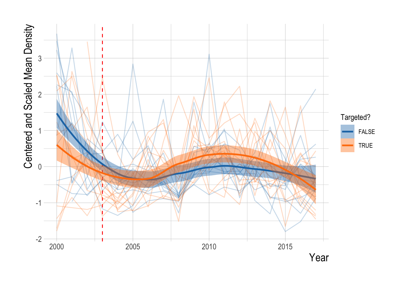
Figure 2.33: Centered and scaled mean annual density, excluding zeros, of included fishes (points) and smoothed means of targeted and non-targeted groups (line) over time

We include a variety of environmental, observation, and temporal indicators in our model. Inclusion of highly co-linear variables in a model can inflate standard errors and obscure “true” effects. To account for this we calculated the Pearson’s correlation coefficients for all of the continuous data included in our model to ensure that none of the included variables had correlation coefficients greater than 0.7, a general rule of thumb for co-inclusion of variables. We did not find problematic levels of correlation among any of our included continuous variables.

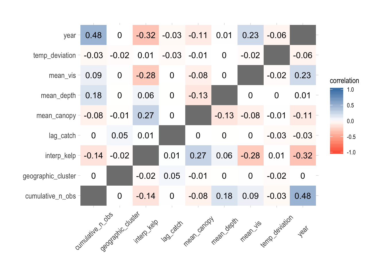
Figure 2.34: Pearson correlation coefficients of continuos data included in the regression model

2.4.2 Selection on Observables

Our proposed identification strategy attempts to control for non-MPA (and not directly modeled) related changes in abundances through the trend in the non-targeted species. However, a simpler alternative would be to simply compare densities before-and-after MPA implementation, while explicitly controlling for non-MPA related factors that we believe may have some effect on densities (a “selection on observables” strategy). To that end, we fit a mixed-effects regression that models log densities (of positive observations only for simplicity’s sake here) as a function of temperature deviations, kelp cover, observer experience, random effects for species and region, and fixed effects for each year in the data (omitting the year 2000).

Using this model, densities of targeted species appear to have been declining steadily since 2000, and appear to have plateaued off since the implementation of MPAs in 2003. Without an identification strategy such as the one employed in this study then, all we could conclude is that densities appear to be lower post-MPA, and have not increased substantially over time (Fig.2.35).

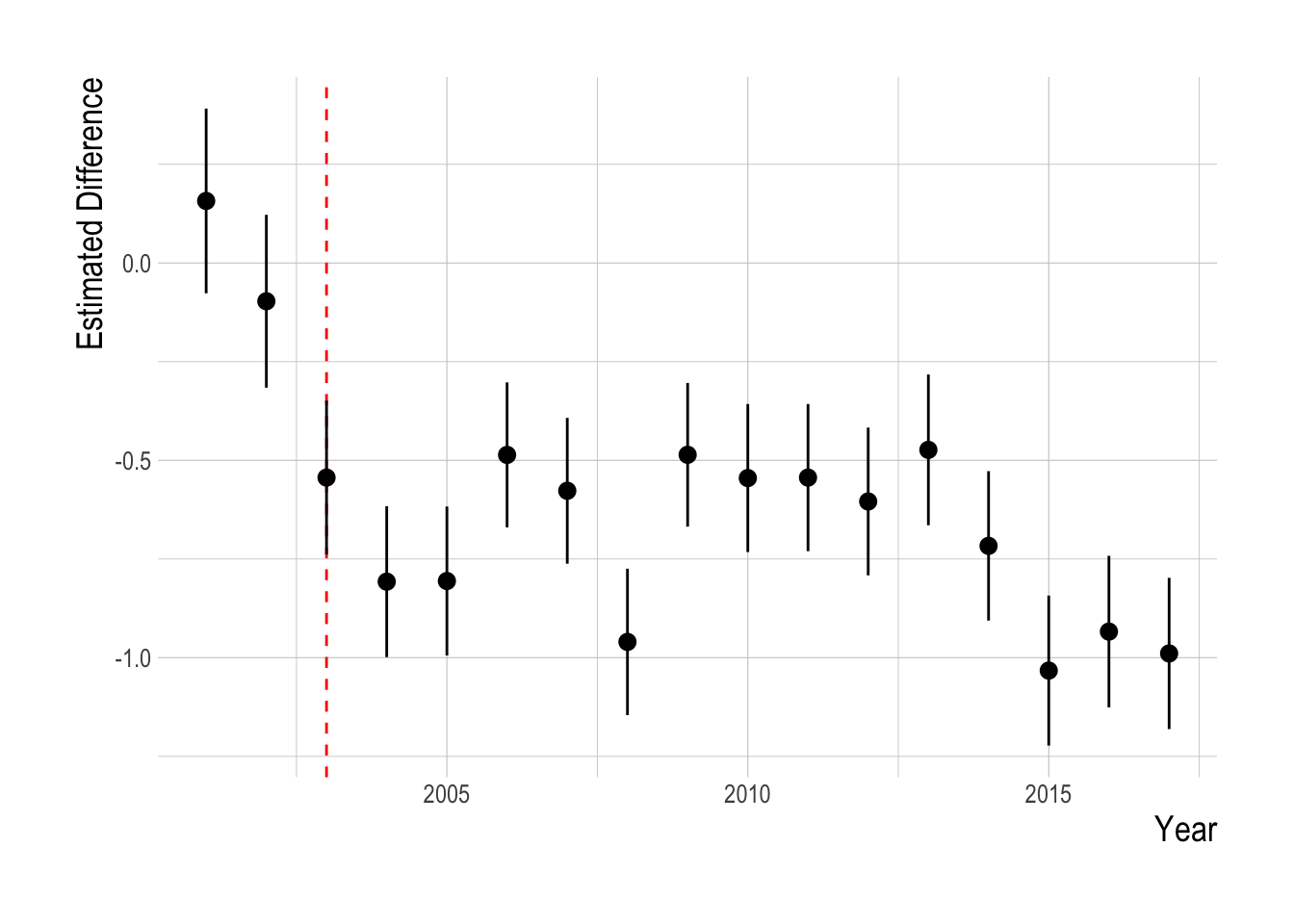
Figure 2.35: Selection on observables identification strategy. Plotted estiamtes are fixed effects of year on log-density (relative to the year 2000), controlling for observer experience, temperature deviations, and kelp cover, with random effects for species and region

2.4.3 Repeat basic analysis.

This analysis has a LOT of complicated moving parts. It’s worth taking a step back and keeping it simple though: what does a simple classic difference in difference analysis say? i.e. targeted + year + year:targeted, aggregating up the densities to take care of the zeros. The results of this basic analysis do tell a different story than our complex über model, indicating broad evidence for a positive regional MPA effect, as measured by the divergence between the targeted and non-targeted. However, we have several reasons to be skeptical of this simplified assessment. First, the error bars are massive here, with effect sizes reaching up to 400%, which our simulation analysis suggests should be unlikely. Second, taking this simplified assessment at face value would suggest that the divergence between the targeted and non-targeted was at near its highest level in 2013, the first year the MPA went in place, suggesting a massive and immediate effect, if we were to take this regression at face value. For these reasons, we do not feel that the simplified regression represents a more accurate result than our mode complete and complex model. Rather, if we simply examine the trend in the simple analysis, rather then the levels, the trend matches our other results (flat, up, and then down). We hypothesize then that our full model acts to 1) vastly reduce the span of the error bars around our estimated divergence between targeted and non-targeted fishes, and 2) remove bias in the effect introduced by covariates (Fig.2.36.

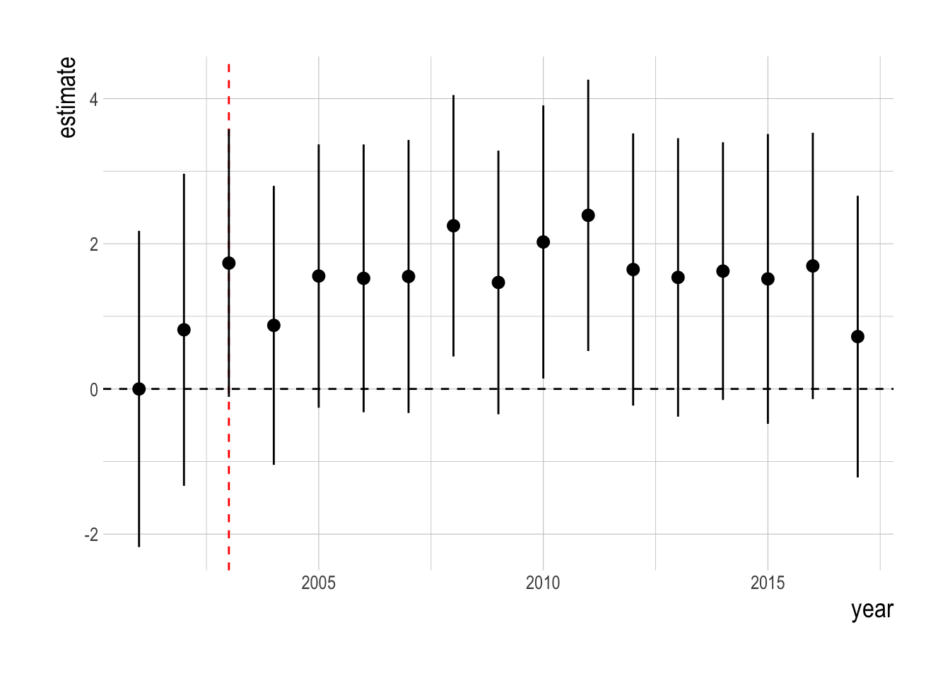
Figure 2.36: Simple DiD using aggregate Density Data

References

Johannes, R.E. (1978) Traditional Marine Conservation Methods in Oceania and Their Demise. Annual Review of Ecology and Systematics 9, 349–364.

Gaines, S.D., White, C., Carr, M.H. and Palumbi, S.R. (2010) Designing Marine Reserve Networks for Both Conservation and Fisheries Management. Proceedings of the National Academy of Sciences 107, 18286–18293.

Halpern, B.S. and Warner, R.R. (2003) Review Paper. Matching marine reserve design to reserve objectives. Proceedings of the Royal Society of London. Series B: Biological Sciences 270, 1871–1878.

Lester, S., Halpern, B., Grorud-Colvert, K., et al. (2009) Biological effects within no-take marine reserves: A global synthesis. Marine Ecology Progress Series 384, 33–46.

Edgar, G.J., Stuart-Smith, R.D., Willis, T.J., et al. (2014) Global conservation outcomes depend on marine protected areas with five key features. Nature 506, 216.

Russ, G. and Alcala, A. (1996) Do marine reserves export adult fish biomass? Evidence from Apo Island, central Philippines. Marine Ecology Progress Series 132, 1–9.

McClanahan, T.R. and Mangi, S. (2000) Spillover Of Exploitable Fishes From A Marine Park And Its Effect On The Adjacent Fishery. Ecological Applications 10, 1792–1805.

Stobart, B., Warwick, R., González, C., Mallol, S., Díaz, D., Reñones, O. and Goñi, R. (2009) Long-term and spillover effects of a marine protected area on an exploited fish community. Marine Ecology Progress Series 384, 47–60.

Halpern, B.S., Lester, S.E. and Kellner, J.B. (2009) Spillover from marine reserves and the replenishment of fished stocks. Environmental Conservation 36, 268–276.

Goni, R., Hilborn, R., D\(\backslash\)’ıaz, D., Mallol, S. and Adlerstein, S. (2010) Net contribution of spillover from a marine reserve to fishery catches. Mar Ecol Prog Ser 400, 233–243.

Kay, M.C., Lenihan, H.S., Kotchen, M.J. and Miller, C.J. (2012) Effects of marine reserves on California spiny lobster are robust and modified by fine-scale habitat features and distance from reserve borders. Marine Ecology Progress Series 451, 137–150.

Thompson, A.R., Chen, D.C., Guo, L.W., Hyde, J.R. and Watson, W. (2017) Larval abundances of rockfishes that were historically targeted by fishing increased over 16 years in association with a large marine protected area. Royal Society Open Science 4, 170639.

Gaines, S.D., Gaylord, B. and Largier, J.L. (2003) Avoiding Current Oversights in Marine Reserve Design. Ecological Applications 13, 32–46.

Botsford, L.W., Brumbaugh, D.R., Grimes, C., et al. (2008) Connectivity, sustainability, and yield: Bridging the gap between conventional fisheries management and marine protected areas. Reviews in Fish Biology and Fisheries 19, 69–95.

Hilborn, R. and Walters, C.J. (1992) Quantitative Fisheries Stock Assessment: Choice, Dynamics and Uncertainty. Springer Science & Business Media.

Gerber, L.R., Botsford, L.W., Hastings, A., Possingham, H.P., Gaines, S.D., Palumbi, S.R. and Andelman, S. (2003) Population Models For Marine Reserve Design: A Retrospective And Prospective Synthesis. Ecological Applications 13, 47–64.

Gerber, L.R., Heppell, S.S., Ballantyne, F. and Sala, E. (2005) The role of dispersal and demography in determining the efficacy of marine reserves. Canadian Journal of Fisheries and Aquatic Sciences 62, 863–871.

Hastings, A. and Botsford, L.W. (2003) Comparing Designs Of Marine Reserves For Fisheries And For Biodiversity. Ecological Applications 13, 65–70.

Hilborn, R., Punt, A.E. and Orensanz, J. (2004a) Beyond band-aids in fisheries management: Fixing world fisheries. Bulletin of Marine Science 74, 493–507.

Hilborn, R., Stokes, K., Maguire, J.-J., et al. (2004b) When can marine reserves improve fisheries management? Ocean & Coastal Management 47, 197–205.

Walters, C.J. and Martell, S.J. (2004) Fisheries ecology and management. Princeton University Press.

Costello, C., Rassweiler, A., Siegel, D., Leo, G.D., Micheli, F. and Rosenberg, A. (2010) The value of spatial information in MPA network design. Proceedings of the National Academy of Sciences 107, 18294–18299.

Fulton, E.A., Bax, N.J., Bustamante, R.H., et al. (2015) Modelling marine protected areas: Insights and hurdles. Phil. Trans. R. Soc. B 370, 20140278.

Gell, F.R. and Roberts, C.M. (2003) Benefits beyond boundaries: The fishery effects of marine reserves. Trends in Ecology & Evolution 18, 448–455.

Russ, G.R., Alcala, A.C. and Maypa, A.P. (2003) Spillover from marine reserves: The case of Naso vlamingii at Apo Island, the Philippines. Marine Ecology Progress Series 264, 15–20.

Harmelin-Vivien, M., Le Diréach, L., Bayle-Sempere, J., et al. (2008) Gradients of abundance and biomass across reserve boundaries in six Mediterranean marine protected areas: Evidence of fish spillover? Biological Conservation 141, 1829–1839.

Vandeperre, F., Higgins, R.M., Sánchez-Meca, J., et al. (2011) Effects of no-take area size and age of marine protected areas on fisheries yields: A meta-analytical approach. Fish and Fisheries 12, 412–426.

Guidetti, P. and Sala, E. (2007) Community-wide effects of marine reserves in the Mediterranean Sea.

Starr, R.M., Wendt, D.E., Barnes, C.L., et al. (2015) Variation in Responses of Fishes across Multiple Reserves within a Network of Marine Protected Areas in Temperate Waters. PLoS ONE 10, e0118502.

Caselle, J.E., Rassweiler, A., Hamilton, S.L. and Warner, R.R. (2015) Recovery trajectories of kelp forest animals are rapid yet spatially variable across a network of temperate marine protected areas. Scientific reports 5, 14102.

Halpern, B.S., Gaines, S.D. and Warner, R.R. (2004) Confounding effects of the export of production and the displacement of fishing effort from marine reserves. Ecological Applications 14, 1248–1256.

Kristensen, K., Nielsen, A., Berg, C.W., Skaug, H. and Bell, B.M. (2016) TMB : Automatic Differentiation and Laplace Approximation. Journal of Statistical Software 70.

R Core Team (2018) R: A Language and Environment for Statistical Computing.

Maunder, M.N. and Punt, A.E. (2004) Standardizing catch and effort data: A review of recent approaches. Fisheries Research 70, 141–159.

Babcock, R.C., Shears, N.T., Alcala, A.C., et al. (2010) Decadal trends in marine reserves reveal differential rates of change in direct and indirect effects. Proceedings of the National Academy of Sciences 107, 18256–18261.

Pershing, A.J., Mills, K.E., Record, N.R., et al. (2015) Evaluating trophic cascades as drivers of regime shifts in different ocean ecosystems. Philosophical Transactions of the Royal Society B: Biological Sciences 370.

Sugihara, G., May, R., Ye, H., Hsieh, C.-h., Deyle, E., Fogarty, M. and Munch, S. (2012) Detecting Causality in Complex Ecosystems. Science 338, 496–500.

Clark, A.T., Ye, H., Isbell, F., Deyle, E.R., Cowles, J., Tilman, G.D. and Sugihara, G. (2015) Spatial convergent cross mapping to detect causal relationships from short time series. Ecology 96, 1174–1181.

Field, J.C., Punt, A.E., Methot, R.D. and Thomson, C.J. (2006) Does MPA mean ‘Major Problem for Assessments’? Considering the consequences of place-based management systems. Fish and Fisheries 7, 284–302.

Roberts, C.M., Bohnsack, J.A., Gell, F., Hawkins, J.P. and Goodridge, R. (2001) Effects of Marine Reserves on Adjacent Fisheries. Science 294, 1920–1923.

Hilborn, R. (2018) Counterpoint to Sala and Giakoumi. ICES Journal of Marine Science 75, 1169–1170.

Sala, E. and Giakoumi, S. (2018) No-take marine reserves are the most effective protected areas in the ocean. ICES Journal of Marine Science 75, 1166–1168.

Cinner, J.E., Maire, E., Huchery, C., et al. (2018) Gravity of human impacts mediates coral reef conservation gains. Proceedings of the National Academy of Sciences, 201708001.

Ovando, D., Dougherty, D. and Wilson, J.R. (2016) Market and design solutions to the short-term economic impacts of marine reserves. Fish and Fisheries, n/a–n/a.

Babcock, E.A. and MacCall, A.D. (2011) How useful is the ratio of fish density outside versus inside no-take marine reserves as a metric for fishery management control rules? Canadian Journal of Fisheries and Aquatic Sciences 68, 343–359.

Thorson, J.T., Munch, S.B., Cope, J.M. and Gao, J. (2017) Predicting life history parameters for all fishes worldwide. Ecological Applications, n/a–n/a.

Punt, A.E., Walker, T.I., Taylor, B.L. and Pribac, F. (2000) Standardization of catch and effort data in a spatially-structured shark fishery. Fisheries Research 45, 129–145.