Chapter 3 Improving Fisheries Stock Assessment by Integrating Economic Theory and Data

3.1 Abstract

The well-being of coastal communities and ecosystems around the world depends on our ability to provide accurate and timely assessments of the status of fished populations. This is typically accomplished by collecting biologically-focused data such as the amount and size of fish captured, and using those data to fit statistical models that estimate factors such as current biomass levels and exploitation rates, usually relative to some benchmark set by stakeholders.

This stock assessment process has had successes throughout the world especially where the data and resources are available to perform what we might call “traditional” statistical stock assessments (Hilborn and Ovando 2014). While many of the world’s largest and most valuable fisheries fall into this category, the majority of people that depend on fisheries do so in smaller scale operations that lack the capacity for traditional stock assessment, a group that has been generally called “data limited fisheries”. This problem has led to an explosion of “data limited stock assessments” (DLAs), that aim to provide management advice using fewer data (but more assumptions). These DLAs have made fisheries assessment possible in previously unassessed places, but increasingly they have sought to simply use more involved statistics to extract more knowledge from the same data (often length composition of the catch).

This study improves the management capacity of data-limited fisheries by demonstrating how expanding the pool of available data to include economic and biological information together can improve the accuracy of stock assessments. While fisheries are coupled socio-ecological systems (Ostrom 2009), the human dimensions of fisheries, the incentives that drive behavior, have been left to economists and other social scientists, while the stock assessment side of the equation has focused on the ecological and biological aspects of a fishery. Our results build off of fisheries economics to show that utilizing data on the economic history of a fishery (prices, costs, technology, labor, and profitability) together with biological data can improve the ability of stock assessment models to accurately estimate fishing mortality rates. In many realistic simulations, we demonstrate that this bio-economic estimation model provides more accurate results than published methods utilizing biological data alone. Lastly, we provide a generalizable simulation framework using machine learning techniques to assess the the relative performance of these models under different states of nature.

Our results demonstrate how often available, but to date underutilized, data can improve stock assessment in data-limited contexts. While we present one specific methodology for incorporating economic data into stock assessment, these results can serve as a foundation for a broader field of study investigating methods for utilizing economic data in biological stock assessment, improving both the accuracy and effectiveness of fisheries management around the globe.

3.2 Introduction

Effective fisheries management requires that managers and stakeholders have some ability to estimate and react to the abundance of fishes in the ocean in a timely manner. The history of fisheries science has been largely concerned with developing and improving our ability to accomplish this difficult task, starting from early models of growth overfishing (as described in Smith 1994) and leading up to multi-species bio-economic models (e.g. Plagányi et al. 2014). While the field has made dramatic advances in our ability to assess the status of fisheries, by and large we have found two solutions to the problems of stock assessment: Fit highly complex integrated statistical models to diverse data streams, or utilize increasing levels of statistical wizardry to try and squeeze more information out of limited data (what has lately been termed Data Limited Stock Assessments, or DLAs). The explosion of DLAs has been both promising and concerning. The majority of fisheries in the world lack the resources for fully integrated stock assessments, and so depend on this world of “data limited stock assessment”. While there has been tremendous growth in this field, nearly all DLAs rely on the same streams of information that would have been available to a fisheries scientist in the 1800s: lengths, captures, and catch per unit effort, generally only one at a time. While these biological data can be highly informative, economic data can also provide information as to the history and status of a fishery. We present here a novel tool for combining historic economic information with traditional fisheries data to improve fisheries stock assessment.

Why do we need a new line of evidence in stock assessment? One could certainly make the case that statistical stock assessments are complicated enough as it is. But, while these “gold standard” assessments (usually) perform well using solely biological data, data-limited stock assessments, in which models are fit by trading in data for assumptions, often struggle if the exact requirements of their assumptions are not satisfied. This can present a major problem for communities and ecosystems that depend on the outcomes of these DLAs to guide their management practices. While future work can examine the usefulness of economic data in a data-rich context, our focus here is in demonstrating how economic information augment biological data to improve the performance of data-limited stock assessments.

What defines a data limited assessment? Dowling et al. (2015) provides a useful summary of what we mean by a data-limited fishery, but for now we can broadly consider data-limited assessments as fisheries lacking sufficient quality information to perform a “traditional” stock assessment, meaning at minimum total catch records and catch-per-unit-effort, on up to a fully integrated statistical catch-at-age model requiring catch, CPUE, length compositions, growth and aging, tagging, etc. A common example of a data-limited fishery would be a fishery for which only CPUE data is available, or for which the only species-specific information are sampled length frequencies from the port or market.

This paper builds off the length-based DLA literature, and so we focus our discussion on the nature of these methods. See Carruthers et al. (2014) and Anderson et al. (2017) for thorough summaries of catch-based DLAs. Length-based DLAs all use life history data or assumptions of some kind to translate the distribution of observed lengths in a fished population into some meaningful management metric. Catch-curves, perhaps the oldest of the DLAs, dating back to at least Chapman and Robson (1960), use assumptions and estimates of the age-at-length relationship to translate lengths into ages, and measure the slope of the logarithm of the numbers at age to provide an estimate of total mortality Z. Assumptions or estimates of natural mortality m can then be used to extract fishing mortality f simply by \(f = Z - m\). Recently, newer methods have evolved that try and estimate fishing mortality rates, recruitment, and selectivity by examining the overall shape of the length composition data (Hordyk et al. 2014; Rudd and Thorson 2017). These models use life history data (or assumptions) to simulate what the length composition of a given population would be expected to be if it were left unfished. This estimate of the unfished length composition is then compared to the observed length composition, and estimates of fishing mortality, recruitment, and selectivity are made that best explain the observed length composition, given the expectation provided by life history data.

3.2.1 What’s the Problem that Economic Data Could Fix?

These existing DLA methods have proven effective and useful in many circumstances, but their reliance on length composition leaves them sensitive to relatively common features in fisheries such as autocorrelated shifts in recruitment regimes. Given length data alone, it is difficult to separate the signal of recruitment from fishing mortality if recruitment is not relatively stable, since both manifest themselves as change in the relative proportions of the observed length classes. The most straightforward solution to this problem is to assume that the population is at equilibrium, and any deviations in expected recruitment are on average zero during the time period of analysis. Year-to-year shifts in the length composition are then attributed to fishing mortality. Given limited data, say only one year of length composition data, this may be the only assumption possible.

Since recruitment regimes are likely to be more the rule than the exception though (Szuwalski and Hollowed 2016; Munch et al. 2018), we would like to be able to relax this key assumption of stable recruitment. Rudd and Thorson (2017) provided an important extension to the equilibrium assumptions underpinning Hordyk et al. (2014) by relaxing the equilibrium assumption and allowing the user to estimate a vector of recruitment deviates and fishing mortality rates given a time series of length composition data. In order to get around the confounded nature of recruitment and fishing mortality, given only length data the LIME model presented in Rudd and Thorson (2017) requires a user specified penalty constraining the amount that fishing mortality can vary year-to-year. More importantly though, LIME provides a flexible tool for integrating multiple forms of data that while still potentially less than what would go into a “traditional” assessment are together still informative. LIME is an important tool for integrating multiple streams of “limited data” together into a comprehensive assessment. However, the data types that can be incorporated into LIME are all components of the traditional fisheries toolbox: lengths, catches, and CPUEs. While these data are important and useful, we present a new model, scrooge, that builds on the foundation provided by LIME to expand the set of possible assessment inputs to include economic theory and data.

Why should we expect economic theory and data to be useful? Fisheries are dynamic bio-economic systems, in which the behavior of fishing fleets affect fish populations, and changes in fished populations affect fishing behavior. This idea was first formalized by Gordon (1954), which sought to explain the evolution of fishing fleets through an open-access model of rent seeking, which results in a fishery reaching an open-access equilibrium where total profits are zero. While this simple model has been vastly expanded on since then, the core idea remains that we can construct models linking human incentives and ecological dynamics to explain fishing behavior.

Bio-economic modeling has most commonly been utilized in the management strategy evaluation (MSE) (summarized in Punt et al. 2016) phase of fisheries management. Early design on management policy centered on identifying the best strategy to employ (e.g. the right size limit or quota), under the assumption that once implemented the policy would be gospel. However, the real world is not often so kind: fishermen respond to incentives and regulations, and therefore what happens on the water is often not what managers had in mind when a regulation was put in place (Salas and Gaertner 2004; Branch et al. 2006; Fulton et al. 2011). As a result of this reality, a growing body of work has sought to build the behavior of fishing fleets into the MSE process, in order to estimate how a policy might actually play out once real people come into contact with it. Nielsen et al. (2017) and van Putten et al. (2012) provide a useful summaries of the large number of models that utilize some form of integrated economic-ecological modeling in the evaluation of management strategies.

Each of these models vary in the structure and complexity with which they model economic behavior, but they share a common feature that they are all focused on the forecasting phase of management, leaving the task of understanding the status of the fishery today to stock assessment models. Thorson et al. (2013) provides one of the only examples of which we are aware of that explicitly incorporates effort dynamics informed by bio-economic theory into the stock assessment process through a state-space catch only model (SSCOM) (though Hilborn and Kennedy 1992 demonstrates the linkages between effort distributions and spatial population structure). Thorson et al. (2013) demonstrates that incorporation of effort dynamics can improve the estimation of biomass from catch data. The model functions by estimating open-access style parameters that serve as aggregate indices of economic conditions in a fishery. However, these economic parameters are not directly informed by economic data; rather priors for these parameters are develop by fitting to observed dynamics of biomass and effort, and these priors are then updated through confrontation with catch data in SSCOM.

In summary, a large body of literature exists showing there exist predictable dynamics between fishing effort and fished populations. Our proposed method builds off this literature in a similar manner to LIME and SSCOM, by hypothesizing that priors informed by economic theory can improve the ability of an assessment model to make sense of limited data. However, we extend this concept to utilize economic data to inform the economic parameters in our model. Specifically, we demonstrate how data on changes in prices, costs, technology, profits, and effort can be utilized to estimate bio-economic parameters that improve the ability of a primarily length-based assessment method to estimate fishing mortality rates.

3.3 Methods

Overview:

• We utilize an age-structured bio-economic operating model to create a database of simulated fisheries

• Fishing mortality rates from the simulated fishery are estimated using scrooge, our bio-economic estimation model

• We assess the performance of different configurations of scrooge using a set of case study fisheries

• We assess broader model performance using a Bayesian hierarchical model and classification algorithms

3.3.1 Why A Bayesian Approach?

Bayesian methods play an important role in fisheries science. Informative priors can help parameterize challenging functions such as the stock-recruitment relationship, and the outcomes of Bayesian assessment provide estimates of posterior probability of states of nature, greatly aiding the management strategy evaluation process (Punt and Hilborn 1997; Myers et al. 2002). While decisions about prior distributions can in some cases dramatically affect assessment accuracy (Thorson and Cope 2017), properly implemented Bayesian methods can provide improved estimates of uncertainty over maximum likelihood approaches (Magnusson et al. 2013).

While there are statistical reasons to favor (and in some circumstances resist) a Bayesian approach to fisheries assessment, our choice of a Bayesian method here is to provide a quantitative framework for bringing local knowledge into the fisheries stock assessment process. To our knowledge, the use of informative priors in data-limited fisheries has focused on biological traits such as growth rates (Jiao et al. 2011) or depletion (Cope 2013), and in general Bayesian processes that make strong use of informative priors (i.e. aren’t just using Bayes for the MCMC) are rare in the data-limited assessment world. We find this general fact somewhat surprising: Bayesian methods can be particularly useful in ecological model fitting when “hard” local data are limited but prior knowledge is available (Choy et al. 2009), as is often the case in data-limited fisheries. In other words, a fishery can be data-limited but knowledge-rich, and a Bayesian process provides a clear statistical framework for incorporating this prior knowledge into the model-fitting process. In addition, it is very common in data-limited contexts to have noisy data that do not paint a clear picture, even after careful statistical analysis. A Bayesian framework allows us to express these uncertain results as posterior probabilities, making statements such as “our model says there is a 75% chance that we are overfishing the population” possible, which are not as feasible in a frequentist setting without approximation methods such as bootstrapping or the delta method. The core hypothesis behind our model is that economic data can inform stock status. While economic data in the form of official government statistics maybe hard to come by, we believe that in these cases economic histories can be elicited from stakeholders. We selected a Bayesian methodology then as an explicit way of bringing this economic knowledge, whether qualitative or quantitative, into the fisheries stock assessment process.

3.3.2 Simulation Model

We simulate different fisheries defined by their biological (e.g. fast vs. slow growing, stochastic vs. deterministic recruitment) and economic (e.g. open-access vs. constant effort) characteristics. Length composition and economic data are then collected from the simulated fishery, and used in our assessment method. Outcomes of the assessment, in this case estimated fishing mortality rates, can then be compared to the true fishing mortality rate experienced by the fishery in that simulation. The simulation model itself is a age-structured single-species bio-economic model, in the form described by Ovando et al. (2016). A given simulation starts by selecting a species. Core life history data for that species (growth, mortality, maturity) are then drawn from the FishLife package in R (Thorson et al. 2017). However, the user can set a number of important specific biological traits for that fishery. For example, the user can specify both the coefficient of variation and autocorrelation of recruitment deviates, and the timing of density dependence (e.g. pre-or-post settlement). On the economic side, for a given simulation the user specifies an initial level of fishing mortality at the start of the fishery, from which dynamics evolve. The effort dynamics are governed by a wide set of specifiable parameters, such as prices, costs, and catchability, all of which can be supplied a coefficient of variation, autocorrelation, and drift. Users also specify the length at 50% selectivity, and the relative profitability of the fishery. The user specifies a fleet model, which can be one of open-access (effort changes in proportion to profit per unit effort in the previous time step), constant-effort (effort stays at the specified initial effort, though fishing mortality rates resulting from this effort can shift if catchability changes over time), or random-walk (effort follows a random walk process from year to year). Across all of these fleet models, users can also specify a coefficient of variation and autocorrelation for deviations from these effort dynamics.

While this operating model is still a large simplification of a real fishery, we incorporate critical traints for evaluating the performance of our assessment model. First, we allow for both recruitment and fishing mortality to shift over time, which will dramatically affect the ability of length-based assessments to perform. Second, we allow for economic data to change over time (e.g. increasing prices), and for these changes to affect the evolution of the fishery through the open-access dynamics model. Third, we can simulate scenarios during which economic data change, but these changes do not translate into changes in effort. In sum then, this operating model allows us to test scenarios that satisfy the assumptions of a biological length-based DLA, that violate those assumptions but satisfy economic assumptions, and that violate both. This provides an diverse sandbox of simulations to test the performance of our proposed assessment method.

3.3.3 scrooge Model

Since our model assumes that fishing behavior is driven by profits, we for call our proposed model scrooge (this probably won’t last in publication, but I like it for now). scrooge can be run using a variety of different combinations of effort process models (e.g. random walk vs open-access) and likelihood structures (e.g. length composition). We use the form economic process model/likelihood components to denote a configuration. For example a configuration of random-walk/lcomp means the model uses a random walk effort process model and includes only length composition data in the likelihood. We assess factorial combinations of process models and likelihoods, omitting combinations that would double count data (e.g. using profit per unit effort data both in the likelihood). See Table.?? for a summary of all of the configuration components.

The estimating model itself was coded in Stan (Carpenter et al. 2017) using the rstan package (Stan Development Team 2018). The core internal operating model is an age structured model identical in structure to the operating model used for the simulations. This means that the model requires user-supplied estimates of life history data, specifically

• Von Bertalanffy growth parameters

• Allometric weight and maturity at length/age equations

• An estimate of natural mortality

• An estimate of Beverton-Holt steepness

We constructed four candidate effort process models describing the effort dynamics of the fishing fleet, and three candidate likelihood structures, each defined by different structural assumptions and data availability. We then fit factorial combinations of each effort process model with each likelihood structure, omitting combinations that would have double counted some information as both a prior and data.

The model has a number of parameters it must estimate, namely fishing mortality rates, recruitment deviates, the length at 50% selectivity, and associated process and observation errors as required (see Table.?? for a complete description of all estimated parameters and their prior distributions). The model is initialized at unfished biomass, and then an estimate of initial fishing mortality is applied for 100 burn-in years, achieving a level of depletion at the start of the data-period of the model. The data period of the model is of length t, and defines the time-steps during which the model estimates dynamic parameters, though the model estimate t + age 50% selectivity recruitment deviates, to allow the model to estimate recruitment pulses which start before the data-period but whose signal can be observed during the early years of the data period. Length-composition data must be available for 1 or more years of the data-period, but are not required in all years. For example, the model can function if given ten years of economic information and only one year of length composition data available at the end of the time period.

All estimation models share common components of recruitment deviates and length composition data. Recruitment is assumed to on average have Beverton-Holt dynamics (Beverton and Holt 1959), reparemeterized around steepness. Process error around this mean relationship is assumed to be log-normally distributed with a bias correction

\[r_{t} = BH(SSB_{t-1},h)e^{r^{dev}_{t}-\sigma_{r}^2/2}\]

\[r^{dev}_{t} = \sigma_rLogRecDev_t\]

\[\sigma_r \sim halfnormal(0.4,0.4)\]

\[LogRecDev_t\sim normal(0,1)\]

Length composition data are structured as discrete numbers of fish counted within one cm length bins per year. While each estimation model differs in its methods for estimating fishing mortality rates, for a given generated mortality rate, vector of estimated recruitment events \(r\), and estimated selectivity \(s^{50}\), the model produces a vector of probability of capture at length \(p^{capture}\) for each time step, given the structural population equations of the model \(g()\).

\[p^{capture}_{t,l} \sim g(f, r, s^{50})\]

The observed numbers at length \(N_{t,l}\) are then assumed to be draws from a multinomial distribution of the form

\[N_{t,1:L} \sim multinomial(p^{capture}_{t,1:L})\]

The key difference in the estimation models is how they estimate f and the data that enter the likelihood. All estimation of f begins by estimating a parameter \(f^{init}\), which is the fishing mortality rate that is held constant over a burn-in period to achieve a given level of depletion by the time of the start of the data period of the model. The estimation models diverge from there in that each specifies a different structural model for how f evolves from \(f^{init}\).

3.3.3.1 Effort Process Models

All effort process model have an expected process and a process error component. The process error, \(E^{dev}\), is estimated in the same manner across all the process models

Effort deviates \(E^{dev}\) are assumed to be log-normally distributed

\[E^{dev}_{t} = \sigma_ELogEDev_t\]

\[\sigma_E \sim halfnormal(0.2,0.2)\]

\[LogEDev_t\sim normal(0,1)\]

The multiplicative effort deviate is then

\[e^{E^{dev}_{t} - \sigma_e^2/2} \]

3.3.3.1.1 Random Walk Model (random-walk)

This estimation model is similar in flavor to the penalty on deviations in fishing mortality used in LIME. The initial effort is calculated as

\[E_{1} = \frac{f^{init}}{q}e^{E^{dev}_{1}-\sigma_{E}^2/2}\]

\[f_{1} = qE_{1}\]

Where q is a catchability coefficient, held at 1e-3.

For the remaining T time-steps, effort evolves as a random walk

\[E_{t} = E_{t-1}e^{E^{dev}_{t}}\]

\[f_{t} = qE_{t}\]

3.3.3.1.2 Bioeconomic Model with Profit Ingredients (ingredients)

We now turn to our class of bio-economic effort models. Across all evaluated bio-economic models, we assume open-access dynamics where fishermen respond to average not marginal profits, per Gordon (1954), which we quantify as profits per unit effort, or PPUE. Under the ingredients model, the user supplies some data on absolute or relative changes in prices p, costs c, and technology (catchability) q, all of which can be thought of as ingredients of profitability. For example, users could report a 25% increase in prices due to the arrival of a new buyer with access to a lucrative foreign market, a 10% decrease in fishing costs due to a government fuel subsidy, and/or a increase in catchability due to the introduction of fish-finder technology. These ingredients of profitability can be provided either as qualitative information or hard data. Any ingredients for which no estimates of relative rates of change are available are assumed to remain constant over the time period of the model. The key feature of this model is that it uses these ingredients to inform our prior estimate of profit per unit effort, \(PPUE_{t}^*\), in a given time step. Therefore, if costs go down and prices go up in a given time step, our estimate of \(PPUE_{t}^*\) will increase appropriately, subsequently increasing our prior on the amount of effort in the following time-step.

Under this model, \(PPUE_{t}^*\) is calculated as

\[PPUE_{t}^* = \frac{p_{t}C(q_{t},B_{t},E_t,s^{50}) - c_{t}E_{t}^2}{E_{t}}\]

where C() represents that Baranov catch equation (Baranov 1918). The revenue part of this profit model is relatively straightforward (price times catch), though it does not allow for factors such as different prices for different size of fish, regardless of weight (e.g. some fish become less valuable as they become larger and no longer fit on plates). The cost equation implies that the “cheapest” units of effort are applied first (e.g. the most skilled fishermen, or the cheapest fishing grounds), and marginal cost of fishing effort increases as more units of effort are exerted (representing less skilled fishermen or costlier fishing grounds). Papers such as Costello et al. (2016) use a cost exponent of 1.27, but in order to keep things simple (and help the simulated fisheries remain stable), we use a value of 2 here. This cost exponent allows us to approximate heterogeneity in fishing costs implicitly without actually modeling fleet components with differing skill.

Notice now that the components price (p), catchability (q), and cost (c) are allowed to vary over time. This is because the model allows for user supplied information on the evolution of these profit ingredients over time, either in the form of actual values (e.g. the price in a given year), or in relative changes (prices are 10% higher than they were last year). For the relative change cases, user supplied inputs are converted to deviations from a mean value and then multiplied by a default mean value set by the model. This is the default for both q and c, since converting user knowledge into the appropriate units is challenging. For a given value of \(PPUE_{t}^*\), we calculate effort in the next time step per

\[E_{t + 1} = (E_{t} + \theta{PPUE_{t}^*})e^{E^{dev}_{t}}\]

where \(PPUE_{t}^*\) is the estimated profit per unit effort, and \(\theta\) sets the responsiveness of effort to \(PPUE_{t}^*\). Note that the model includes the same effort process error as utilized in the random-walk process model. So, the profit ingredients and the open-access assumptions provide our prior on the effort in a given time step, but we estimate potential deviations from this prior expectation. From there, the fishing mortality in a time step is calculated as

\[f_{t} = q_{t}E_{t}\]

One difficulty in this process is that the dynamics of the open access model are driven by the relative profitability of the fishery, and as such largely to the relative scale of revenue and costs. Therefore, getting the relative magnitude of prices and costs to be correct is important. Unfortunately, while prices can be relatively easily determined, costs are much more difficult to obtain, especially in units matching the exact effort units of the operating model. To solve this problem, we estimate an additional parameter in this estimation model, \(c^{max}\). The cost in any time is then calculated as

\[c_t = c^{max}c^{rel}\]

where \(c^{rel}\) are the relative costs (scaled as deviations from a mean) over time t supplied by users. \(c^{max}\) itself is tuned in a rather long process that results in much cleaner estimation that can actually be provided with informative priors. Rather than estimating \(c^{max}\) itself, we estimate a cost-to-revenue ratio at the start of the fishery. We first estimate a guess of, given the simulated nature of the fishery, something close to maximum revenues (assumed to come by fishing a bit harder than natural mortality when the population is completely unfished). We then calculate the profits associated with these maximum revenues given a prior estimate of the cost to revenue ratio CR.

\[PROFITS^{max} \sim MAX(PRICE)CATCH^{B0}(1 - CR) \]

Given this estimate of \(PROFITS^{max}\), we can then back out the cost coefficient \(c_{max}\) that, given the other parameters, would produce those profits. Estimating the cost to revenue ratio instead of the actual costs allows for informative priors to be set. A fishery that at its heyday was incredible profitable will have a low cost to revenue ratio, while a fishery that was scrapping by on its best day would have a high cost to revenue ratio.

While the prior can be informed from local stakeholders, we set a zero truncated normal prior on the cost ratio of

\[CR \sim halfnormal(0.5,1)\]

The other challenging parameter in the open access equation is \(\theta\), the amount that effort changes for a one unit change in \(PPUE\). Similarly to estimating the cost to revenue ratio instead of raw costs, rather than estimate \(theta\) directly, we estimate the maximum percentage change in effort from one time step to the next. As part of the cost to revenue tuning process, we estimated the maximum profits, and the effort that would produce those profits. Together that provides us with the maximum expected PPUE. For a given max percentage change (\(\Delta^{max}\)) in effort then, we calculate \(\theta\) as

\[\theta = (\Delta^{max} E^{MAX}) / PPUE^{MAX}\]

While \(\theta\) has no intuitive sense for most stakeholders, the maximum percentage year-to-year change in effort can be elicited from stakeholders. For now, we assume a zero truncated normal prior on the max expansion

\[\Delta^{max} \sim halfnormal(0,0.25)\]

The ingredients effort process model allows us to utilize provided ingredients of profitability to drive our prior expectations of the dynamics of fishing effort. Importantly, our translation of complex parameters such as cost coefficients or the marginal effect of PPUE on effort into interpretable parameters such as cost to revenue ratios and maximum percent changes in effort greatly improves the ability of users to elicit informative priors from stakeholders in real-world applications of this method (Choy et al. 2009).

3.3.3.1.3 Bioeconomic Model with PPUE Data (ppue)

The ingredients model makes use of individual components of profitability, under the theory that a) these data are informative to the evolution of effort and b) these data may be easier to obtain than for example actual mean profitability across the fishery. However, we can also consider an effort process model in which PPUE is assumed to be known. While complete knowledge of average PPUE in a fishery is unlikely, especially in a data-limited context, survey methods could be constructed to collect estimates of PPUE, which being a central part of a fisherman’s business, is not an unreasonable piece of information to think could be obtained, given the right questions and sufficient trust (acknowledging that PPUE will likely have many and more of the challenges in interpretation as CPUE data; e.g. Walters 2003).

So, the the ppue model, rather than estimating \(PPUE_{t}^*\) as a function of its ingredients, we simply take collected values of PPUE as data, and estimate effort per

\[E_{t + 1} = (E_{t} + \theta{PPUE_{t}})e^{E^{dev}_{t}}\]

We estimate \(\theta\) using the same methods described in the ingredients method (estimating the maximum percent change in year-to-year effort instead of \(\theta\) directly).

Since we no longer assume knowledge of technology changes over time, we assume a static q. This assumption could be relaxed in future model runs to consider knowledge of both PPUE and technology, but for now we make this assumption to make a cleaner distinction between the ingredients model and the other models.

\[f_{t} = qE_{t}\]

3.3.3.1.4 Effort Data Model (effort)

Both of the bio-economic process models (ingredients and ppue) model the change in effort as a function of profit per unit effort. Their key function, from the perspective of a model focused on estimating biological fishery metrics, is to help inform estimates of time-step-to-time-step changes in fishing mortality. To follow the old adage “keep it simple stupid”, we also build a model that assumes data on the time-step-to-time-step proportional changes in fishing effort. While such data are unlikely to be available for a fishery covering a large and diverse geographic range, for more localized small-scale fisheries such knowledge is not unreasonable. For example, fishing cooperatives in Chile often maintain data on fishing effort.

Under the effort process model, we assume knowledge of the proportional changes in effort over time \(\Delta^{effort}\), where

\[\Delta^{effort} = E_{t+1}^{true}/E_{t}^{true}\]

and

\[E_{t + 1} = (E_{t}\Delta^{effort})e^{E^{dev}_{t}}\]

and

\[f_{t} = qE_{t}\]

3.3.3.2 Likelihood Models

The effort process models represent alternative hypotheses as to the true operating model driving the evolution of fishing effort, and partly by extension fishing mortality, in a fishery. In other words, the economic process models inform our prior on the evolution of effort. However, a central motivation of this research is to diversify both the data available to our assessment operating models (as we have done with the use of economic data as components of Bayesian priors), and the data with which we confront these models. The traditional core pantheon of data with which we confront models in fisheries are abundance indices (derived from either fishery dependent or independent sources) and length/age composition data. We propose to add profit per unit effort and proportional changes in effort to this group, at least as a starting point in the data-limited context of this study.

3.3.3.2.1 PPUE as an Index of Effort (lcomp+ppue)

We consider catch-per-unit-effort to be informative in fisheries (on a good day) through the relationship

\[CPUE_{t} = \frac{q_{t}E_tB_t}{E_t} = q_tB_t\]

A constant or time-varying estimate of q then is our link between an observed CPUE data and an unobserved state of nature, \(B_t\) that we wish to estimate.

We propose a similar use for profit per unit effort, but rather than PPUE informing an index of abundance, it serves as an index in the rate of change in effort (and by extension conditional on q), fishing mortality. If we assume that a standard open-access dynamics model is true, then

\[E_{t + 1}^{true} = E_{t}^{true} + \theta{PPUE_{t}}\]

Simply rearranging this equation, we can provide a link between PPUE and the change in effort as

\[PPUE_{t} = \frac{E_{t + 1}^{true} - E_{t}^{true}}{\theta^{true}}\]

We can therefore use PPUE as an index of the change in time-step-to-time-step effort. In other words, given that our model estimates \(E\) through one of our process models,

\[PPUE_{t}^* = \frac{E_{t+1} - E_{t}}{\theta}\]

\(\theta\) is estimated in the same manner as outlined in the economic process models, and from there we can utilize \(PPUE\) in the likelihood per

\[PPUE_{t} \sim normal(PPUE_{t}^*,\sigma_{obs})\]

Remember though that in our models we are estimating \(E_{t}\). The above likelihood is only identifiable if we either provide a constraining prior on the evolution of \(E_{t}\) (as all of our effort process models do) and/or include other components to the likelihood, which we do by fitting to the length composition data in all runs (otherwise the model could estimate a vector of efforts that predict PPUE perfectly). In other words, when we include \(PPUE_{t}\) in the likelihood, the model estimates a vector of efforts that maximize the likelihood of both the PPUE and length composition data, conditional on the prior probabilities assigned to the evolution of effort by our effort process model.

It is also worth noting that by including \(PPUE\) in the likelihood, we are now including both process error (quantified as \(\sigma_E\) in the estimated effort deviates) and observation error (\(\sigma_{obs}\)), in a similar manner to the methods outlined in Thorson and Minto (2015), though the Bayesian nature of our analysis makes it hierarchical rather than “mixed effect” in nature, since all variables are random in a Bayesian setting (Gelman et al. 2013). Given the data constraints, we are only able to identify both process and observation error by providing constraining priors on our estimates of both.

Our prior for \(\sigma_{obs}\) is a zero-truncated normal distribution with a user-specified CV

\[ \sigma_{obs} \sim halfnormal(0, CV^{PPUE}\frac{1}{T}\sum_{t = 1:T}{PPUE_{t}})\]

3.3.3.2.2 Index of Effort Changes (effort)

Trying to keep it simple one last time, in our effort process model, we assumed knowledge of the relative change in effort over time. Rather then than fitting to an index of the change in effort, we can simply fit a model to the change in effort data, assuming some observation error.

\[\Delta^{effort} \sim normal(\frac{E_{t+1}}{E_{t}}, \sigma_{obs})\]

This likelihood model follows the same identification constraints as the PPUE model.

3.3.3.3 Simulation Testing

We simulation tested factorial combinations of these process models and likelihood forms (omitting combinations that double count data, e.g. pairing the ppue process model with the length+ppue likelihood model) using a single species age-structured bio-economic operating model. For each run of the model, a species of fish, and its associated life history data, was randomly selected from the database provided by Thorson et al. (2017). The only stochastic process in the biological model are (potentially) autocorrelated a drifting recruitment deviates. For that run, a fleet model is also chosen from one of three options

• open-access
  • fishing effort responds to profit per unit effort, governed by chosen values and dynamics of price, cost, q, the the change in effort per unit of PPUE
• constant-effort
  • fishing effort is held constant at some initial value
• random-walk
  • fishing effort evolves through a random walk behavior

For all of these fleet models, the user specifies the degree of variation, autocorrelation, and drift for prices, costs, and catchability. The selected parameters are used to simulate a fishery over a 100 year period. For each time step, length composition data are sampled from the fisheries catch using a multinomial distribution, assuming a CV of the length-at-age key of 20%.

We simulated two case studies for this paper; an open access model which while containing noise still conforms to the open-access dynamics central to much of the assessed models assumptions, and a random-walk model in which while economic data are still collected, change in effort are completely unrelated to changes in economic conditions. Along with these case studies, we also simulated 200 fisheries, each with random draws of the simulation parameters (e.g. species, fleet model, degree of variation and drift of economic parameters).

For every simulated fishery, we then stipulated a range of the data to sample, and a combination of a process model and a likelihood structure to fit scrooge to those data. In this study, we sampled length composition and economic data for a period of up to 15 years during the middle of the simulated fishery’s evolution. Within this 15 year window, we consider two cases, one where length composition data are available for all 15 years, and another where while economic data are available for all 15 years, length composition data are only available for the last four years of the time series. We then pass the chosen model configuration, data and associated life-history parameters to scrooge to fit the model. This results in 3800 simulations (20 model configurations of 200 simulated fisheries, less 200 simulations that producsed nonsensical results (fishing mortality rates consistently above 10 or below .01)).

For now, we focus on estimation of fishing mortality rates. As the model also estimates selectivity, given assumptions about the spawning biomass at age, it is simple to also estimate and present common metrics such as the spawning potential ratio (SPR). However, for brevity’s sake here, we focus on demonstrating the potential of the model to estimate fishing mortality f. In addition, we do not consider observation error at this time. While this is clearly not a remotely realistic choice, we made this decision due to the novel nature of the the integrated use of economic data and dynamics into the stock assessment process. If scrooge is unable to provide substantial improvements (or actually provides worse estimates) than a standard lengths-only assessments model, in the form of Rudd and Thorson (2017) or Hordyk et al. (2014), even with perfect information, then it is unlikely to do well with imperfect knowledge. However, future testing will clearly need to address this step, which our operating model is already capable of incorporating.

3.3.3.4 Model Comparison

We focused on two variables for model comparison: root median squared error (RMSE) and bias in the (up to) most recent five years of the data. For every run of our model we obtained i iterations of t estimates of fishing mortality rates from our HMC chain. For each iteration i, we then calculated the RMSE and bias as

\[rmse_{i} = sqrt(median((predicted_{i,t} - observed{i,t})^2))\]

and bias as

\[bias_{i} = median(predicted_{i,t} - observed_{i,t})\]

There are many other potential metrics for use, but we focus on these since the units are interpretable, since both the median and bias are in units of fishing mortality rates, which we can reasonably consider along a range of ~ 0 to 2. We could also compare estimates such as median relative error, which expresses the median percentage error of a given iteration. While this is useful, we felt that, given the potential low values of fishing mortality this metric could be misleading at times. For example, suppose that the true fishing mortality rate is 0.05, and we estimate a fishing mortality rate of 0.1. The MRE for this case would be 100%. But, if the true fishing mortality is 0.5, and we estimate 0.55, our MRE would only be 10%. But, from a management perspective, the two are, we would argue, equally accurate, which RMSE captures. By calculating RMSE and bias in terms of absolute (rather than relative) deviations, we can provide managers with a sense of whether the expected uncertainty for a given model spans a large or small range of fishing mortality rates.

We use RMSE and bias to assess the performance of scrooge in our case studies. We also used RMSE to provide a higher level summary of overall and context specific performance of the candidate scrooge models. To judge overall performance, we fit a hierarchical Bayesian model to our simulated fits, in which the dependent variable is RMSE, and the independent variables include simulation characteristics such as the degree of recruitment variation, the degree of variation in economic parameters, the life history of the species, and hierarchical effects for each scrooge model. This model then provides posterior probability estimates of the average effect of each candidate scrooge model on RMSE, controlling for covariates.

This method provides estimates of overall model performance, but it is likely that different scrooge models will perform best under different circumstances. To examine this possibility, we fit a decision tree model using the rpart function implemented in the caret package, where the dependent variable is, for each simulated fishery, the best (in terms of RMSE) scrooge model, and the independent data are the simulation characteristics. This method provides an algorithm for deciding on the best scrooge model configuration given the characteristics of a fishery.

Lastly, we also used LIME to estimate fishing mortality for each of the 3800 simulated assessments scenarios, and then for each scenario calculated the difference in RMSE resulting from LIME and scrooge

3.4 Results

3.4.1 Case Studies

Each scrooge model configuration is defined by the economic process model and the likelihood. We describe these in the text as economic process model/ likelihood model. So, a model using the random-walk economic process model and just length composition data would be random-walk/lcomp. A model using random-walk and length composition and PPUE data in the likelihood would be random-walk/lcomp+ppue.

All case studies examine the performance of a scrooge model fit using the radom-walk fleet model and only length composition data in the likelihood (random-walk/lcomps), to a scrooge model with an open-access economic process model informed by data on prices, costs, and technology, and a likelihood comprised of length composition data and PPUE (ingredients/lcomp+ppue). We chose these two scrooge configurations to illustrate the use of no-economic data vs. the use of both open-access dynamics, profit ingredients, and PPUE data.

For the first case study, we consider a scenario where 15 years of length composition and economic data are available, and the underlying dynamics contain stochasticity and drift in recruitment and economic parameters, but satisfy the open-access assumptions of the scrooge model utilizing economic data. In this case, both the random-walk/lcomps and ingredients/lcomp+ppue models estimate the rough magnitude of fishing mortality over the span of the data. However, the random-walk/lcomps model misses the slow upward trend in fishing mortality in the most recent years. The ingredients/lcomp+ppue model incorrectly estimates that a large upward spike in fishing mortality occurred in year four, but captures the upward trend in fishing mortality rates over the last five years of the data. RMSE and bias were both nearer to zero for the ingredients/lcomp+ppue model over the last five years of the data (Fig.3.1).

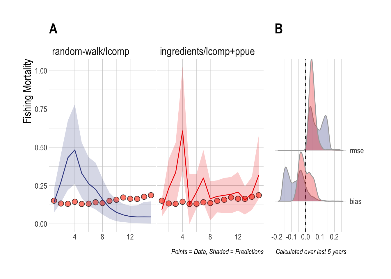
Figure 3.1: Case Study 1 A) True fishing mortality (points) and estimated mean (line) and 90% credible intervel (ribbon) of fishing mortality. Filled red points indicate that length composition data were available during that time step. B) Posterior distribution of RMSE and bias (colors map to ribbon colors in A)

This first case study is useful both in demonstrating the performance effects of utilizing economic data in stock assessments, and in highlighting the challenge with fitting to length composition data that addition of economic data can help overcome. The random-walk/lcomp and ingredients/lcomp+ppue models in (Fig.3.1) present very different pictures of the history and state of this fishery: The random-walk/lcomp only model presents a fishery in decline, while the ingredients/lcomp+ppue model describes a fishery with an increasing trend in fishing mortality. However, the fits of each of these models to the length composition data are nearly identical (Fig.3.2). In other words, from the perspective of the length composition data alone, both of these stories are almost exactly as equally likely, with the random-walk/lcomp model utilizing recruitment deviates more than changes in effort to explain shifts in the length composition data. The ingredients/lcomp+ppue model, in the form of data on prices, costs, and q incoming our open-access process model and on the PPUE data used in the likelihood, simply assigns greater posterior probability to a state of the world explaining the recent length composition less through recruitment and more through changes in fishing mortality.

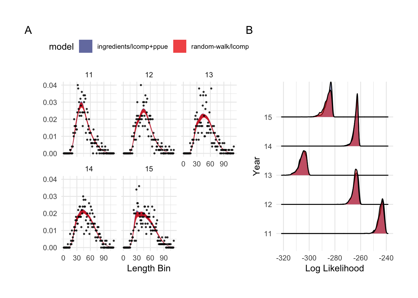
Figure 3.2: Observed and predicted 90% credible interval of case study length composition data (A, note that they overlap almost perfectly), and log-likelihood of length composition fits by scrooge configuration (B)

The second case study is identical to the first, except that now length composition data are only available for the final three years of the evaluation period. The results are very similar to the first case study; the ingredients/lcomp+ppue model is able to capture the recent upward trend in fishing mortality, while the random-walk/lcomp cannot (Fig.3.3).

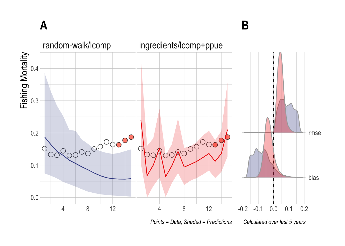
Figure 3.3: Case Study 2 A) True fishing mortality (points) and estimated mean (line) and 90% credible intervel (ribbon) of fishing mortality. Filled red points indicate that length composition data were available during that time step. B) Posterior distribution of RMSE and bias (colors map to ribbon colors in A)

The first two case studies demonstrate that the ingredients/lcomp+ppue configuration is capable of outperforming, in terms of RMSE and bias, the random-walk/lcomp configuration that does not leverage economic information. This should be expected though: through the prior we are feeding the model more information about the operating model, and since we do not incorporate observation error at this time and since the dynamics of the simulation model in this case match the dynamics of scrooge’s operating model, we would hope that more data = better results. In an ideal world, we would want scrooge to perform better when its assumptions are satisfied, and to not perform dramatically worse when its assumptions are not.

To address this, for the third case study we fit the same scrooge configurations to a simulation in which effort is completely decoupled from profits (effort evolves through a random walk), but data are still collected on economic components of profits (prices, costs, technology, and PPUE). While the random-walk/lcomps model ignores these data, the ingredients/lcomp+ppue model uses these data, and the associated assumption of open-access dynamics, in its fitting procedure. In this case, the 90% credible interval estimated by the random-walk/lcomps model now covers the upward trend in fishing mortality, though the mean estimated trend is flat. Despite using incorrect assumptions, the ingredients/lcomp+ppue model still manages to outperform the lengths only model (Fig.3.4).

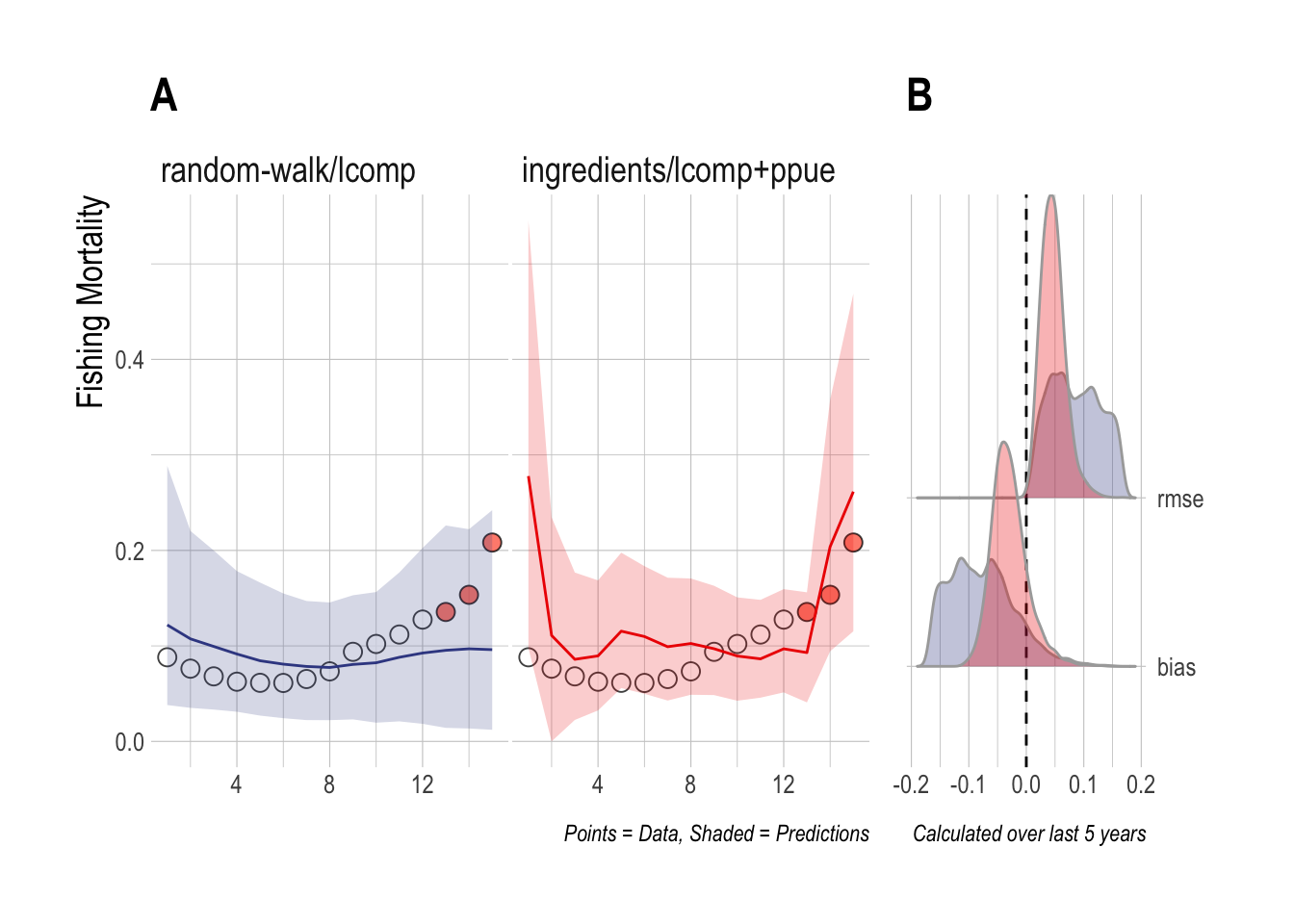
Figure 3.4: Case Study 2 A) True fishing mortality (points) and estimated mean (line) and 90% credible intervel (ribbon) of fishing mortality. Filled red points indicate that length composition data were available during that time step. B) Posterior distribution of RMSE and bias (colors map to ribbon colors in A)

3.4.2 Overall Model Performance

The case studies provide visual and quantitative evidence that the introduction of economic data and theory through the scrooge model can improve estimates of fishing mortality over utilizing length composition data alone. Those were three simple examples though, out of a vast array of possible states of nature a fishery might experience. We used a Bayesian hierarchical modeling routine to provide an overall performance estimate for each of the scrooge configurations tested here (defining performance as the effect of a given configuration on RMSE over the last five years of the data). This model allows us to estimate, all else being equal, which model will reduce the RMSE of our estimates of fishing mortality the most.

scrooge models incorporating data on the percentage change in effort in the process model (effort), or the likelihood (lcomps + effort) provide the greatest expected reduction in RMSE. Models utilizing profit ingredients (ingredients) (data on prices, costs, technology) in the open-access operating model show some evidence of actually on average increasing RMSE, while models utilizing PPUE in the process model or the likelihood showed uncertain effects on RMSE (Fig.3.5)

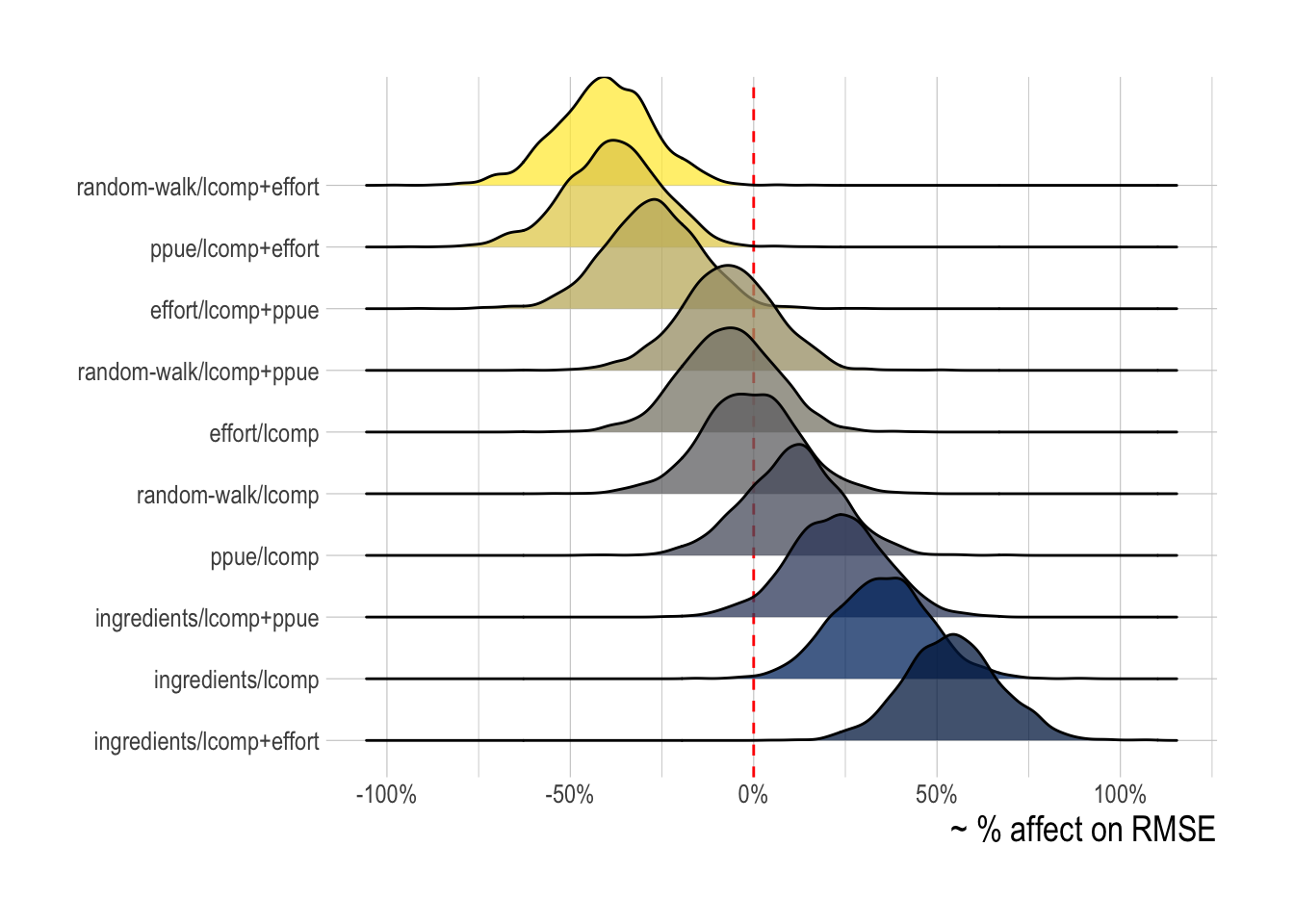
Figure 3.5: Posterior probability distributions of the effect of each tested scrooge configuration on log(RMSE). Fill illustrates mean change in RMSE

While this hierarchical analysis gives evidence that some models may on average indeed perform better than others, for any one simulated fishery different scrooge configurations may be best. To test this idea, for each simulated fishery we chose the scrooge configuration that provided the lowest RMSE over the last five years of the data, allowing us to see the frequency with which different configurations were selected (Fig.3.6). As would be expected from the mean expected model performance, the models utilizing data on the percentage change in effort in the process model or likelihood were most frequently selected. A model containing some form of economic data and/or theory (i.e. not random-walk/lcomps) was selected nearly in nearly 100% of model runs.

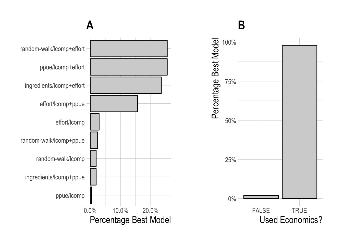
Figure 3.6: Frequency of selection for each individual scrooge configuration (A), and grouping by utilization of economic data or not (B)

Our results so far suggest that we would overwhelmingly prefer to have access to data on the the relative change in effort over time to include our data-limited assessment. This though should come as no surprise: Trends in effort are directly proportional to trends in fishing mortality, unless catchability changes substantially over the time period (or effort and catchability vary substantially throughout the fleet). While we include trends and deviations in catchability in the simulation models, under the rates of change of catchability simulated in our model, effort is still a good proxy for the evolution of fishing mortality. So, feeding the model data on effort should perform well.

While the inclusion of effort data is interesting to consider, it is likely to be impractical in many data-limited fisheries. We do not consider observation error here, but unlike say PPUE, in order to be useful the trend in the effort data is not a property of the mean effort but rather the total effort in a fishery. This means that we would need to be able to obtain an estimate of the changes in total effort throughout the fishery, an unlikely task in any but geographically small or relatively data-rich fisheries. Collection of a sample of changes in effort could be strongly biased, in terms of its link to fishing mortality, if for example a few large high-liners are not included in the data. In contrast, profits per unit effort, and the ingredients of PPUE, are sample estimates, meaning that we care what average PPUE is in the fishery, not total. So, even if we miss a few extremely profitably (or unprofitable) fishermen, if we sample well we can get an estimate of the mean PPUE.

Given this, we re-ran our model selection process, but omitting any scrooge configurations that utilize data on the percentage change in effort. Configurations utilizing PPUE in the likelihood were the most frequently selected, but closely followed by models utilizing only length data, though models utilizing profit ingredients in the economic process model were still selected some of the time. Overall, models incorporating some form of economic data or theory were selected across approximately 75% of simulated fisheries.

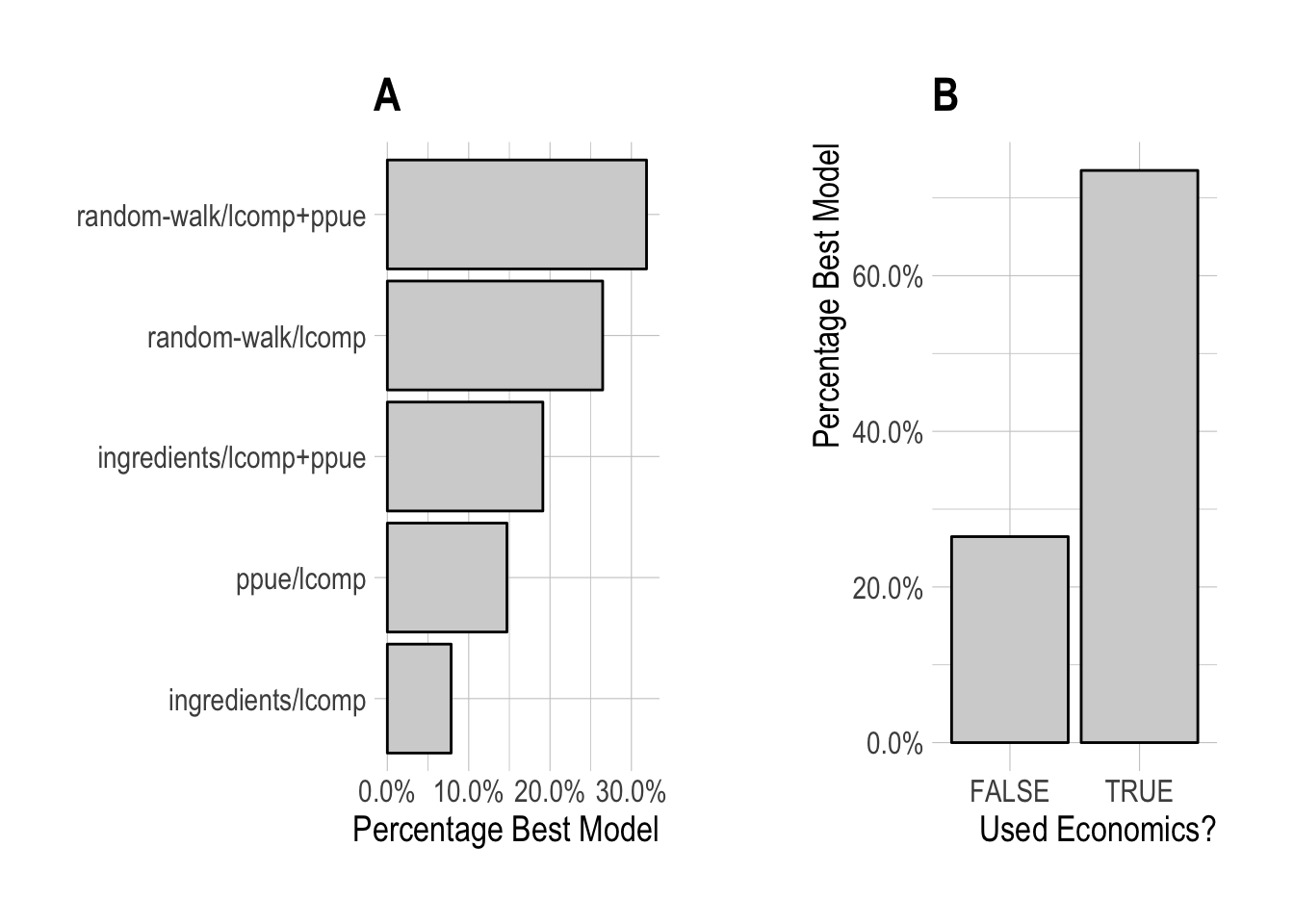
Figure 3.7: Frequency of selection for each individual scrooge configuration, (A), and grouping by utilization of economic data or not (B), omitting any configurations using effort data

These results show that while some scrooge configurations, i.e. process model types and likelihood structures, are more commonly selected than others, nearly every evaluated configuration was selected on occasion. For a user then, the selection of a scrooge configuration can be a daunting task. To facilitate model selection, we used our simulated data to construct a decision tree algorithm for selecting the appropriate scrooge configuration. For each simulated fishery, we identified which configuration minimized RMSE over the last five years of the data. From there, we trained the decision tree to these selected configurations to develop a decision tree do determine a scrooge configuration based on the characteristics of the simulated fishery. For all of these runs we ignore configurations using effort data, since our earlier results say that if you have it, use it.

While further work will need to be conducted to translate this tree into user-supplied variables, our results show for example that if you know nothing about the fishery, the best choice is to assume a random walk economic process model while utilizing PPUE in the likelihood. But, if prices have been increasing substantially, then the model utilizing a bio-economic model with profit ingredients as the process model and PPUE in the likelihood may be best (ingredients/lcomp+ppue). Alternatively, if prices are not increasing and recruitment is not highly autocorrelated, then it may be best to ignore economic data in the assessment (Fig.3.8). This is an illustrative example of what would need to be a more involved simulation test, but demonstrates the ability of simulation testing and machine learning techniques to facilitate decision making. Importantly, the decision tree process does provide some measure of confidence in a given node by pointing out the relative proportion of the true decisions that fell into each bin. So for example, if the decision tree says to use random-walk/lcomps, but examining the fit this was true 51% of the time in the data, and ingredients/ppue was selected the other 49%, then this suggests that we should not put a lot of weight in choosing one over the other in this case.

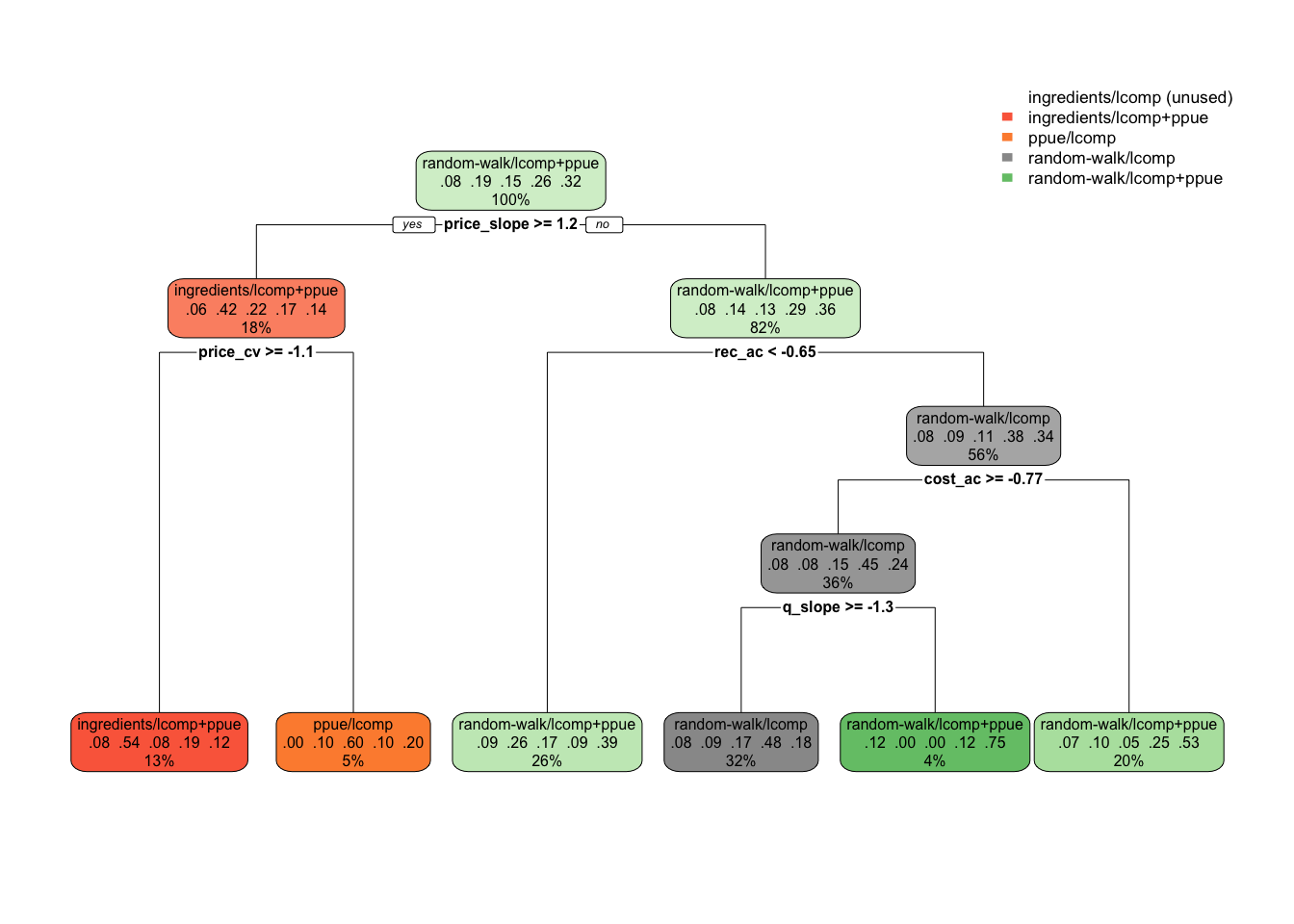
Figure 3.8: Decision tree suggesting scrooge configurations as a function of fishery characteristics (omitting configurations using effort data). Decimal numbers show proportions of the data that fell into that classifcation at that node, percentages the percent of observations at a given level that fall in that node

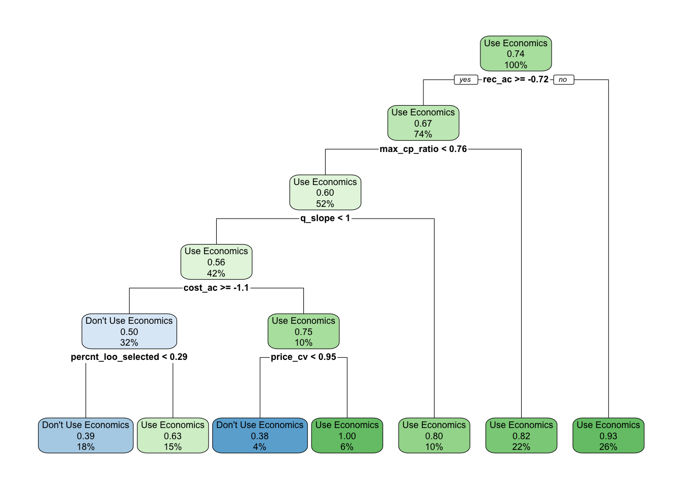
Figure 3.9: Decision tree recommending Use / Don’t Use economics in assessment. Decimal numbers show proportions of the data that fell into that classifcation at that node, percentages the percent of observations at a given level that fall in that node

3.4.3 Comparisons with LIME

All of our analyses so far have been internal to the scrooge model. These results demonstrate that scrooge is capable of using economic data to improve estimates of fishing mortality. How does it compare though to other models that utilize length composition data to estimate fishing mortality rates, such as LIME (Rudd and Thorson 2017)? As a preliminary assessment of this question, we used LIME to estimate fishing mortality rates from our 3800 simulations, using only the length composition data. In these circumstances, LIME does not estimate a process error around fishing mortality, but rather estimates fishing mortality as a fixed effect, with a penalty on the year-to-year changes on estimated fishing mortality. For consistencies sake, we set our prior on the process error for fishing mortality in scrooge to the same value as the penalty used in LIME (0.2). Both models receive the exact same data.

Comparing the two models, we see that inclusion of economic information through scrooge more frequently resulted in improved estimates of fishing mortality (as measured in reductions in root mean squared error) than those produced by LIME, though LIME did outperform scrooge during many runs, especially in cases where scrooge utilized profit ingredients in the open-access process model (Fig.3.10). Interestingly, the scrooge configuration that utilizes length composition only in the likelihood and a random walk for the economic process model (random-walk/lcomps) is more or less the exact same model that LIME uses, and yet the scrooge version of this model provided lower RMSE than LIME in approximately 80% of the simulations (Fig.3.10). Further research is needed to determine if this is a result of the priors utilized in scrooge, or due to some inherent performance trait of fitting through Hamiltonian Monte Carlo in Stan vs through maximum likelihood with the Laplace approximation in TMB, or simply a house effect of both the simulation model and scrooge being written by the same author.

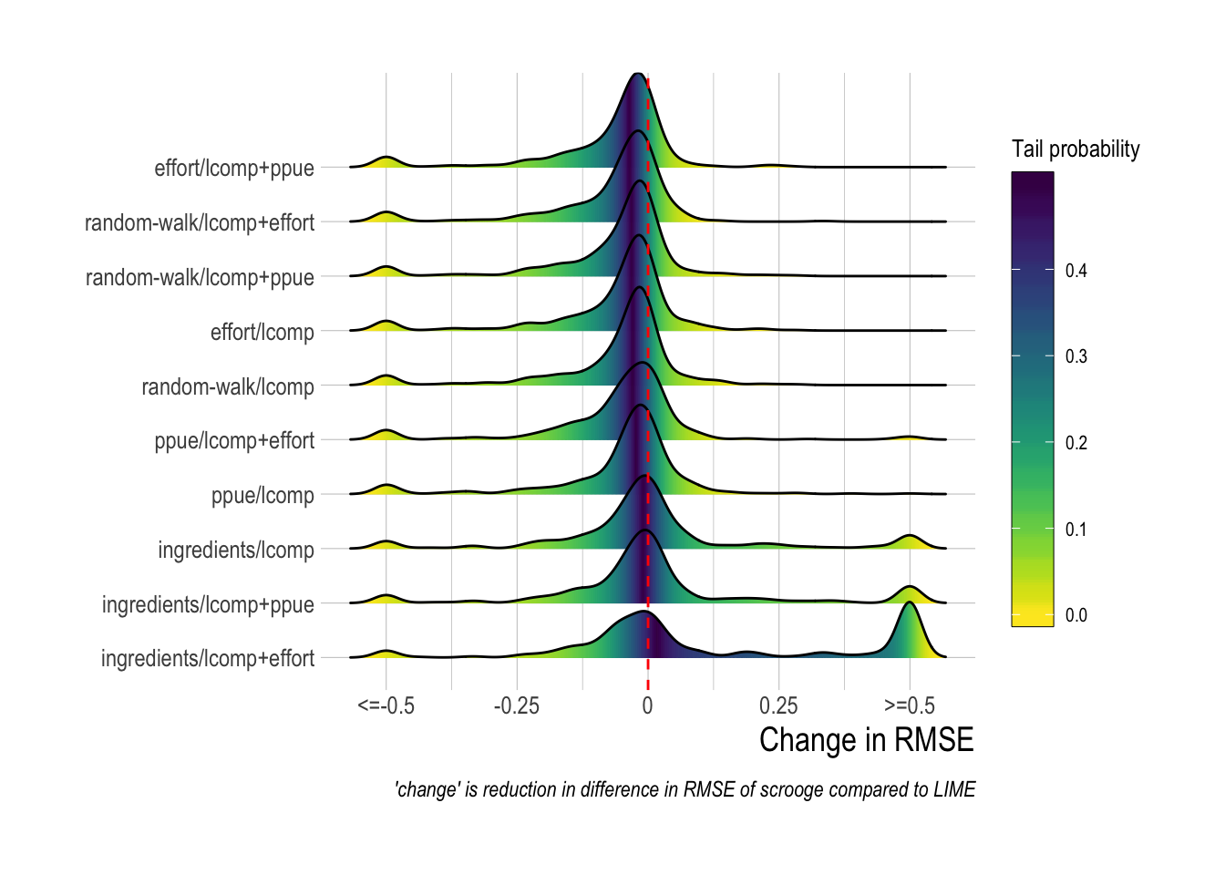
Figure 3.10: Distributions of difference (scrooge - lime) root median squared error across simulated fisheriess. Values are capped at differences of |0.5|, which represnts a substantial difference in performance when fishing mortality is commonly on the scale of 0 to 2

3.5 Discussion

Fisheries management is a complicated task far a large and varied range of reasons, most centrally the incentives of a common-pool resources, the challenges of placing individual species in an ecosystem context, and the sheer logistical and statistical difficulties in estimating the abundance and exploitation of fish populations whose adults and larvae can cover vast distances while being subjected to a host of environmental drivers. The aim of this study is to demonstrate how integration of economic data and theory can make this problem of estimating status less challenging under the right circumstances. We find that while different kinds of economic information can be useful under different contexts, across our simulated fisheries inclusion of economic data almost always improved our ability to estimate fishing mortality. Our results provide a clear and novel path for the integration of an underutilized form of information in fisheries stock assessment.

Looking narrowly at scrooge, the length-and-economics DLA proposed here, there are several limitations that must be addressed. Most critically, we do not yet address observation error. We feel that this is justified given the novel nature of the concept proposed here; as a first phase we have demonstrated that, given perfect information, economic data can substantially improve the performance of a length-based data-limited assessment. The critical next step will be to ask, how accurate does economic data utilized in this assessment have to be to remain beneficial? Luckily, this modeling framework makes this a simple task, the only barrier being resources for a much larger number of simulated fisheries and assessments. Beyond that, and similar to most other DLAs, we do not incorporate important but challenging factors such as time-varying and/or environmentally driven growth and mortality, or multi-species interactions. Under a data-limited context, these choices are likely to be inevitable, but the addition of more data in the form of economics opens up potential spaces for identification of more parameters such as these (or at least to assess the ramifications of ignoring these states of nature).

From the fleet perspective, we do not yet address the complexities of multiple fleets or time-varying and/or dome-shaped shaped selectivity. We make this choice to make presentation of our initial results tractable, but future investigations can relatively easily incorporate these factors. Broadly, there are many challenges to consider in utilizing a new source of data. Catch-per-unit-effort data at its face seems like an obvious indicator of stock status, and yet a whole body of literature has evolved documenting when it is and is not a useful index (Hilborn and Kennedy 1992; Walters 2003; Maunder and Punt 2004). Similar efforts will need to be conducted if for example profit per unit effort is to be broadly incorporated in data-limited assessments. But, economic theory combined with our simulation tool can help with this process by examining when and how much PPUE data helps or hurts under increasingly realistic scenarios.

Our results show that accurate data on the percentage changes in total fishing effort are likely to provide the greatest reduction in root median squared error. If these data are not reliably available though, we find that the choice of which model is “best” is highly dependent on the characteristics of a specific fishery. Future work and theory may identify an emergent set of cases where one particular model configuration is preferable. As the number of assessment methods increases, and the range of fishery scenarios in which we we want to run assessment diversify, relying on qualitative rules of thumb is likely to become more challenging though, unless a small set of assessments emerge as overwhelming favorites. We propose the pairing of large-scale simulation testing with classification algorithms to help resolve this problem. On their own, this process allows the data to inform us which models are likely to perform well under a particular set of circumstances. Further work is needed to translate characteristics of simulated fisheries into parameters that users could reliably understand. These methods could also serve as the underpinning for ensemble assessment approaches, such as those presented by Anderson et al. (2017), that rather than picking one model generate an aggregate output based on predictions of each model weighted by their expected accuracy under given circumstances. We recognize that this approach may seem as a “black box”, and we would encourage users not blindly trust algorithm outputs. At a minimum, for such a tool to be useful it would have to inform users as to how similar their particular fishery is to the simulated library of fisheries on which the decision algorithm is based. But, we feel that the use of theory and empirical approaches such as these can make the process of deciding which model to use when easier and, properly done, more transparent, if paired with an iterative process of careful consideration by users (why do we think the model is picking a given assessment in this case)?

In a similar vein, comparisons between scrooge and other assessments such as LIME are in no way intended to establish a “best” assessment. Our results show that, under the very specific set of circumstances simulated here, inclusion of economic theory and data through scrooge often outperformed, in terms root median squared error, estimation by LIME using only length-composition data in the likelihood. However, we also found many cases where LIME outperformed scrooge (Fig.3.10). Similar to the decision tree method we used to for model selection within scrooge, we can also start using this simulation testing method to develop decision tree across models. Two areas of particularly interesting research will be a) how flawed economic data and/or assumptions can be before its inclusion becomes useless or actively harmful and b) comparison of lengths + economic data to for example lengths + CPUE, or lengths + CPUE + PPUE.

Looking more broadly, there are several important challenges to the integration of economic knowledge in stock assessment that need to be addressed. Open-access dynamics are central to all of the scrooge configurations except those that assume some knowledge of the percentage changes in effort in the fishery over time. This clearly begs the question, how would this model work in a quota managed, limited-entry, or rationalized fishery? If effort is constrained by both regulation and profits, profits alone may not be informative. While we do not test these scenarios here, we a) could incorporate them to the simulation framework but more importantly b) can use this assessment as a foundation for thinking about how to integrate economic knowledge from fisheries with different types of effort dynamics and incentive structures into the assessment process. For example, in rationalized fisheries, data on the price and dynamics of quota trading could be informative as to fishery perceptions of stock status. While these are real concerns, as a starting place though we feel that assuming open-access dynamics is a reasonable assumption for many data-limited fisheries in which we would envision using the scrooge assessment model as envisioned here. Similar to the evolution of economic behavior in the MSE process, we begin with simple open-access models of effort dynamics to illustrate this process. These simple models may indeed by accurate for some fisheries (perhaps especially those for which we do not have sufficient data to identify these dynamics), but are certainly not an appropriate model for many fisheries (Szuwalski and Thorson 2017). However, future research can begin to incorporate more complex and realistic models of fishing behavior from the wealth of studies examining the dynamics of fishing fleets (Vermard et al. 2008; e.g. Marchal et al. 2013).

We also casually suggest that data such as trends in prices, costs, technology, effort, or profit per unit effort be accurately collected and utilized in the assessment process. Our results show that, in theory, collecting these data is likely to be worth it from the perspective of assessment accuracy (though a full cost-benefit management strategy evaluation would be needed to assess the tradeoffs in assessment accuracy with the costs of data collection, as discussed by Dowling et al. 2016). Why do we feel that these data may be obtainable in a data-limited contexts, where more traditional fisheries data such as total removals are not? The first is that fishermen can talk while fish cannot. In our experience, fishing stakeholders often have detailed knowledge on the economic history of their fishery. While future work is needed to determine the best strategies for translating this knowledge into the form required by scrooge, this is a surmountable challenge (Choy et al. 2009). Second, governments or stakeholders that have not had the capacity or interest in collecting historic fisheries data may still have official records on data related to the fishing industry, including fuel prices, government subsidies, export prices, and changes in wages. We are under no illusion that obtaining the types of economic data utilized by scrooge will be simple, but our results show that it is worth determining how best to obtain and use these data. One fascinating area of future research will be considering the relative value of information of each of the profit “ingredients”, e.g. how valuable, from an assessment accuracy perspective, is price data relative to technology data?

While Bayesian analysis has a strong tradition in fisheries science, informative priors have rarely been used in data-limited fisheries assessment, with notable exceptions such as Cope et al. (2015) and Jiao et al. (2011). Our analysis provides a quantitatively rigorous method for integrating prior knowledge on the economic dynamics of a fishery into the assessment. While we would argue that appropriate informative priors can be useful in data-limited or data-rich contexts, in a data-limited context they can be particularly useful, especially where they allow for local knowledge that does not fit neatly into the traditional fisheries data bins to be included. An important feature of our model is that nearly all of the priors utilized in our model are interpretable by users. For example, rather than requiring users to provide a prior, in the appropriate units, for the responsiveness of effort to a one-unit change in profit per unit of effort, we instead allow users to provide a prior on the most that effort is likely to expand from one year to the next. Priors for parameters such as the standard deviation of recruitment can be drawn from appropriate literature. In addition, the Bayesian nature of our model allows users to specify the degree of confidence that should be assigned to prior beliefs or data. If for example estimates of profit per unit effort are believed to be highly questionable, we can increase our prior on the magnitude of observation or process error in the model.

The simplest case for integrating economic data would be finding troves of actual unused data, for example data on historic ex-vessel prices. However, in many real world applications this will not be the case (e.g. a database of cost to revenue ratios is likely to be rare) requiring elicitation of priors on these parameters from stakeholders. Properly eliciting these priors from stakeholders will be challenging. However, a rich literature exists on designing robust prior elicitation methods, and since our simulation results suggest that economic priors can be a useful component of stock assessment, we can now consider real-world practicalities of obtaining robust priors for model parameters (see Choy et al. 2009 for a thorough summary of this process in ecology).

The use of informative priors in fisheries stock assessment can be concerning for some users. The stock assessment process is (ideally) directly tied to management outcomes, and so the results of an assessment can be extremely important to different stakeholders, from conservation interests to fishermen. A reasonable critique of using informative priors then is that different groups could easily tip the results of an assessment in their favor by providing priors that make their desired outcome more likely. While this is a real issue, we feel that the relative benefits of including informative priors in data-limited assessment (in this case through economic theory and data) outweigh these potential risks. Beyond the general fact that non-Bayesian methods have just as many opportunities for “subjective” decision making, the Bayesian process we propose here would require stakeholders to translate their beliefs into quantifiable metrics that they would then have to defend. A user desiring to manipulate an outcome by assigning a strong probability of no overfishing even at open-access equilibrium would have to present and defend an extremely high cost to revenue ratio in that fishery. This position would be difficult to defend if the fishery is know to have been or currently be highly profitable to other stakeholders. This Bayesian process can make outright gaming through unreasonable priors more transparent, not less. In addition, in a real-world application, any priors included in the model would have to be elicited before any model fitting was done. This prevents scenarios such as retroactively adjusting priors once the results of an assessment are known. This process also allows for informative discussion post-model fitting. If results do not match prior expectations, we can use this process to show users what attributes of the data are causing this mismatch, allowing users to see that while their beliefs were incorporated, the data have more support for another outcome. Broadly, incorporation of informative Bayesian priors in data-limited assessment is a complicated process that can be solved (Choy et al. 2009), and we argue that in doing so we can produce more accurate assessment outcomes and improve stakeholder relations by providing a clear mechanism for incorporating their local knowledge into the statistical assessment.

The dynamics of fisheries are dictated in part by the interplay of economic incentives and ecological constraints. Natural resource management, and fisheries in particular, have gone a long way towards understanding these dynamics, from simple theories of open-access dynamics to agent-based multi-species models. While we have increasingly used this understanding to project the likely consequences of policy choices (as summarized by Nielsen et al. 2017), we have yet to broadly utilize these dynamics in the assessment phase of fisheries management. While methods such as SSCOM, described in Thorson et al. (2013), utilize economic theory to help inform fisheries assessment, to our knowledge this study is the first to incorporate this theory with data on the dynamics of economic incentives to create an integrated bio-economic stock assessment model. We find that integration of economic information can substantially improve the accuracy of fisheries stock assessment, allowing in this case users from a data-limited context to utilize local fishery knowledge to improve their ability to effectively manage their marine resources. Our hope is that this research can serve as a foundation for a broader field of inquiry linking economic behavior with biological knowledge to improve our knowledge of the state of global fisheries.

3.6 Supplementary Material

It is not feasible to provide in-depth fitting diagnostics for all 3800 simulated assessments. However, we can broadly report that the percent of divergent draws across all simulations was less low (generally less than 1%), as were the percentage of draws that exceeded the maximum treedepth.

To provide some diagnostics of model fitting, we can examine key HMC diagnostics for our third case study (the hardest of the case studies for scrooge to fit), to verify that under these circumstances our model converges properly. Standard divergence, energy, and treedepth diagnostic plots were created with the bayesplot package.

Figure 3.11: Energy plot of Case Study 3. Delta energy histogram closely matches energy, suggesting fat tails are not a problem

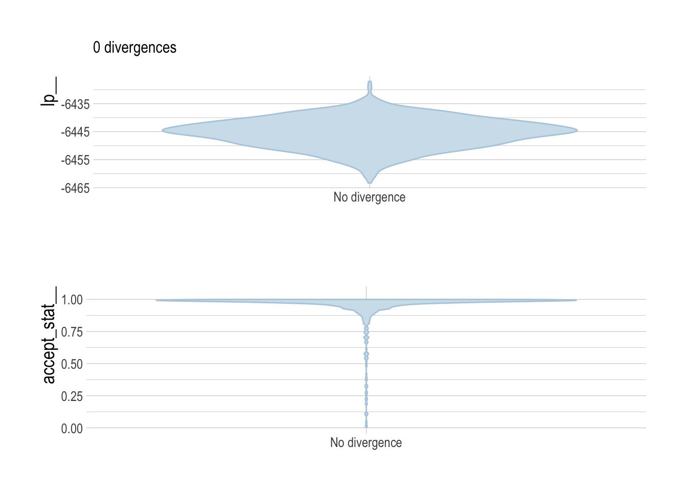
Figure 3.12: Log posterior and acceptance stat as a function of divergence. No runs were divergent

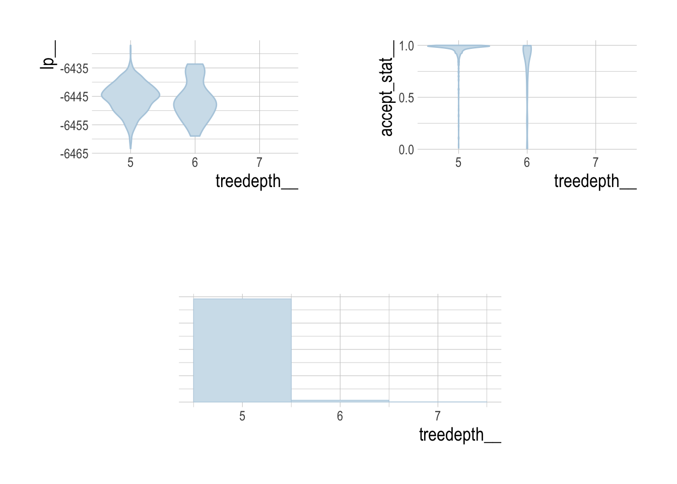
Figure 3.13: Log posterior, acceptance stat, and counts of treedepth. Max treedepth was set to 12, which no runs exceeded

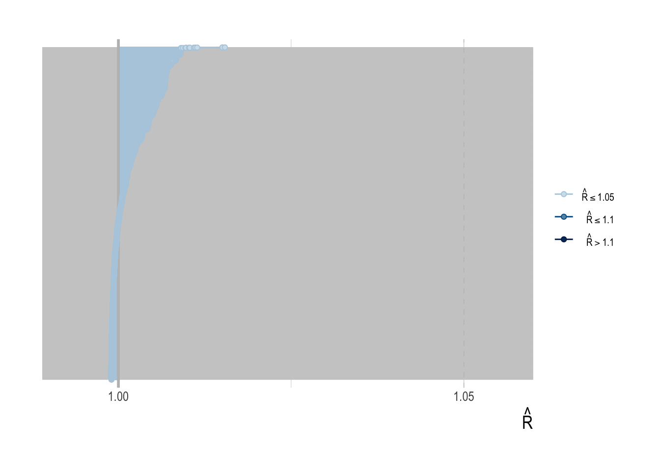
Figure 3.14: Rhat diagnostic for all estimated parameters. No parameteres exceeded 1.05, meaning there is not clear evidence of insufficient effective sample sizes for any parameters

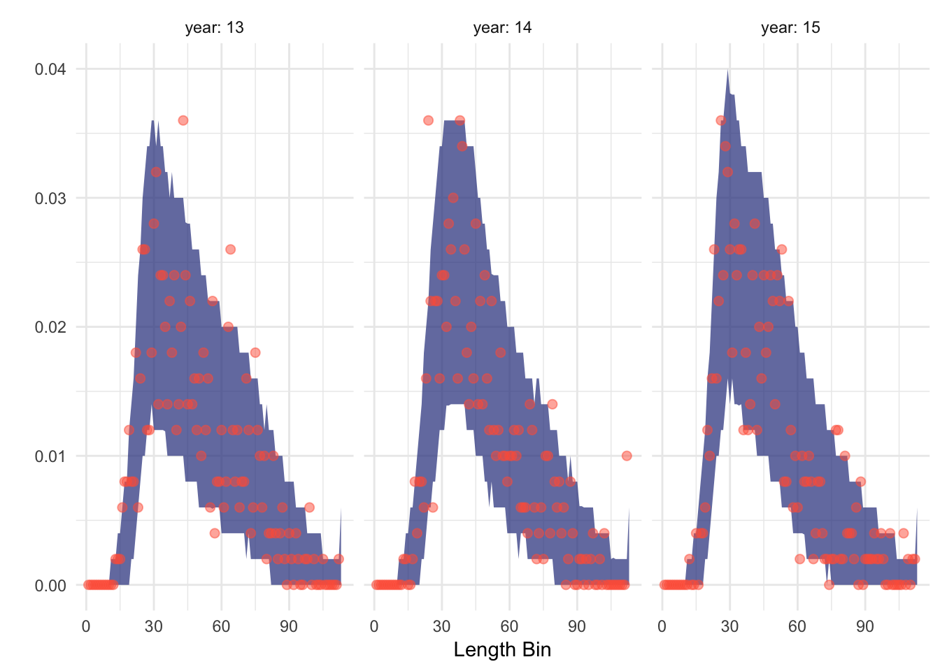
Figure 3.15: 90% pospterior predictive distribution (shaded ribbon) of fitted length composition data (points). Nearly all observed points fall within the 90% bounds of the posterior predictive distribution

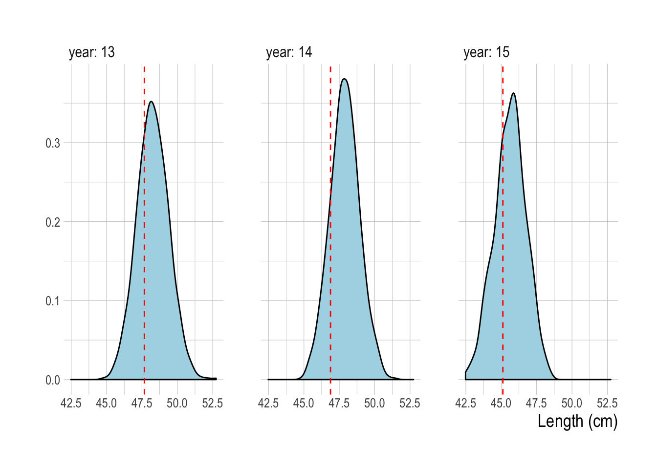
Figure 3.16: 90% Posterior predictive credible intervals of mean length (distribution) and observed mean length (red line) over time. True mean lengths all fell within posterior predictive distribution

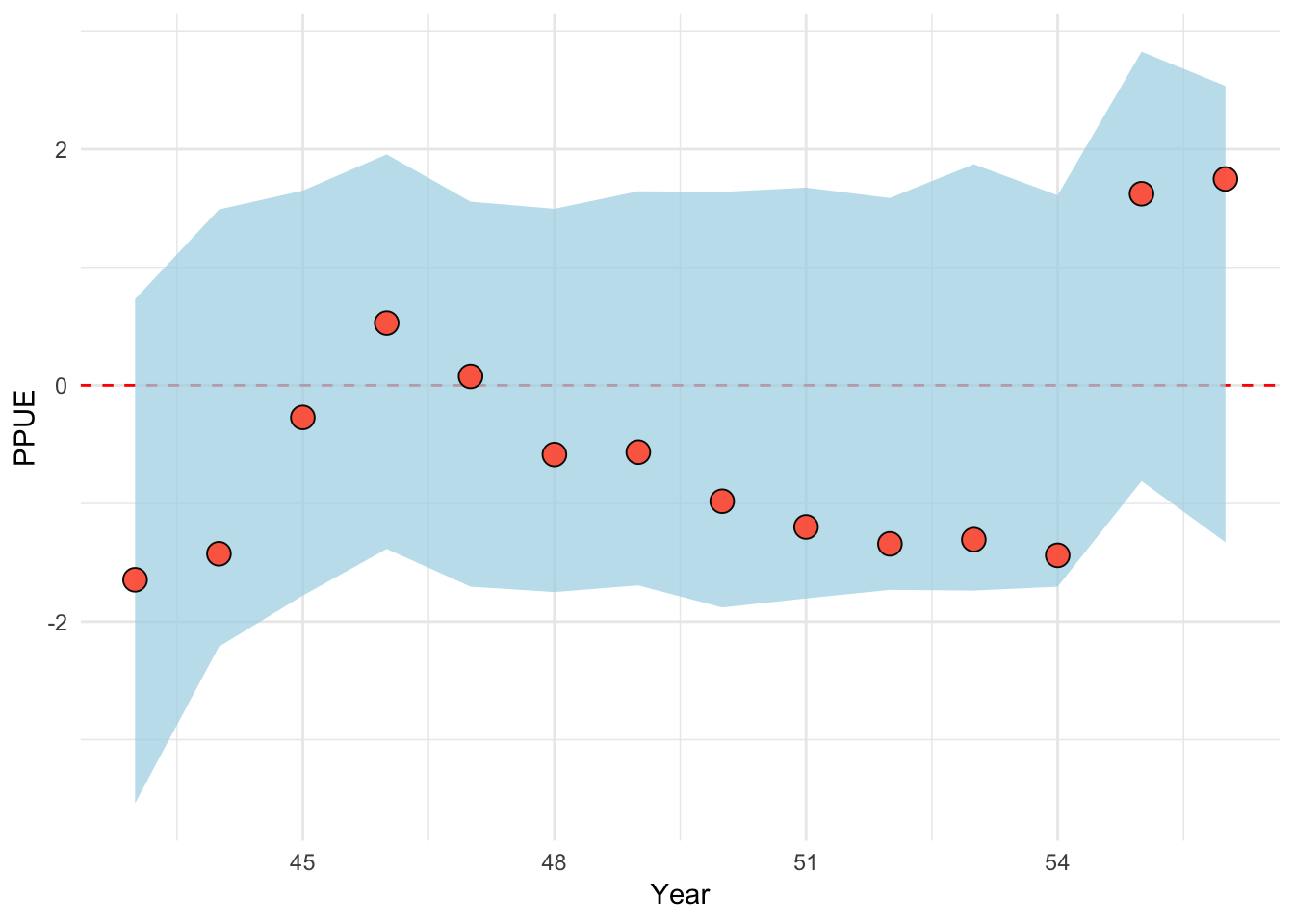
Figure 3.17: 90% credible interval of posterior predictive draws of profit per unit effort (ribbon), and observed profit per unit effort (points)

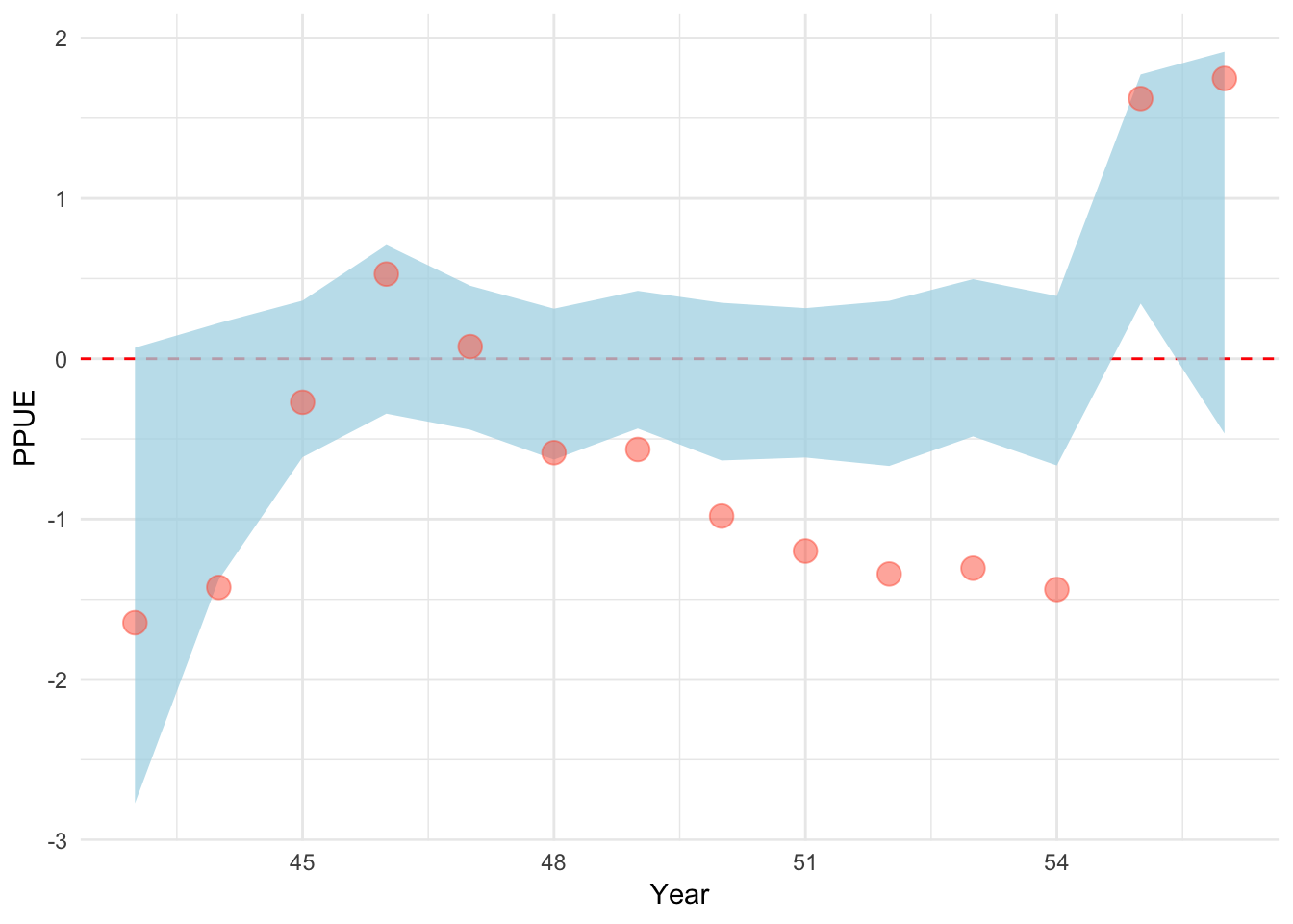
Figure 3.18: 90% credible interval of posterior probability distribution of profit per unit effort (ribbon), and observed profit per unit effort (points)

References

Hilborn, R. and Ovando, D. (2014) Reflections on the success of traditional fisheries management. ICES Journal of Marine Science: Journal du Conseil 71, 1040–1046.

Ostrom, E. (2009) A General Framework for Analyzing Sustainability of Social-Ecological Systems. Science 325, 419–422.

Smith, T.D. (1994) Scaling fisheries: The science of measuring the effects of fishing, 1855-1955. Cambridge University Press.

Plagányi, É.E., Punt, A.E., Hillary, R., et al. (2014) Multispecies fisheries management and conservation: Tactical applications using models of intermediate complexity. Fish and Fisheries 15, 1–22.

Dowling, N.A., Dichmont, C.M., Haddon, M., Smith, D.C., Smith, A.D.M. and Sainsbury, K. (2015) Guidelines for developing formal harvest strategies for data-poor species and fisheries. Fisheries Research 171, 130–140.

Carruthers, T.R., Punt, A.E., Walters, C.J., MacCall, A., McAllister, M.K., Dick, E.J. and Cope, J. (2014) Evaluating methods for setting catch limits in data-limited fisheries. Fisheries Research 153, 48–68.

Anderson, S.C., Cooper, A.B., Jensen, O.P., et al. (2017) Improving estimates of population status and trend with superensemble models. Fish and Fisheries 18, 732–741.

Chapman, D.G. and Robson, D.S. (1960) The Analysis of a Catch Curve. Biometrics 16, 354–368.

Hordyk, A., Ono, K., Valencia, S., Loneragan, N. and Prince, J. (2014) A novel length-based empirical estimation method of spawning potential ratio (SPR), and tests of its performance, for small-scale, data-poor fisheries. ICES Journal of Marine Science: Journal du Conseil, fsu004.

Rudd, M.B. and Thorson, J.T. (2017) Accounting for variable recruitment and fishing mortality in length-based stock assessments for data-limited fisheries. Canadian Journal of Fisheries and Aquatic Sciences, 1–17.

Szuwalski, C.S. and Hollowed, A.B. (2016) Climate change and non-stationary population processes in fisheries management. ICES Journal of Marine Science 73, 1297–1305.

Munch, S.B., Giron‐Nava, A. and Sugihara, G. (2018) Nonlinear dynamics and noise in fisheries recruitment: A global meta-analysis. Fish and Fisheries 0.

Gordon, H.S. (1954) The economic theory of a common-property resource: The fishery. The Journal of Political Economy 62, 124–142.

Punt, A.E., Butterworth, D.S., Moor, C.L. de, Oliveira, J.A.A.D. and Haddon, M. (2016) Management strategy evaluation: Best practices. Fish and Fisheries 17, 303–334.

Salas, S. and Gaertner, D. (2004) The behavioural dynamics of fishers: Management implications. Fish and Fisheries 5, 153–167.

Branch, T.A., Hilborn, R., Haynie, A.C., et al. (2006) Fleet dynamics and fishermen behavior: Lessons for fisheries managers. Canadian Journal of Fisheries and Aquatic Sciences 63, 1647–1668.

Fulton, E.A., Smith, A.D.M., Smith, D.C. and van Putten, I.E. (2011) Human behaviour: The key source of uncertainty in fisheries management. Fish and Fisheries 12, 2–17.

Nielsen, J.R., Thunberg, E., Holland, D.S., et al. (2017) Integrated ecological–Economic fisheries models—Evaluation, review and challenges for implementation. Fish and Fisheries, n/a–n/a.

van Putten, I.E., Kulmala, S., Thébaud, O., Dowling, N., Hamon, K.G., Hutton, T. and Pascoe, S. (2012) Theories and behavioural drivers underlying fleet dynamics models. Fish and Fisheries 13, 216–235.

Thorson, J.T., Minto, C., Minte-Vera, C.V., Kleisner, K.M. and Longo, C. (2013) A new role for effort dynamics in the theory of harvested populations and data-poor stock assessment. Canadian Journal of Fisheries and Aquatic Sciences 70, 1829–1844.

Hilborn, R. and Kennedy, R.B. (1992) Spatial pattern in catch rates: A test of economic theory. Bulletin of Mathematical Biology 54, 263–273.

Punt, A. and Hilborn, R. (1997) Fisheries stock assessment and decision analysis: The Bayesian approach. Reviews in Fish Biology and Fisheries 7, 35–63.

Myers, R.A., Barrowman, N.J., Hilborn, R. and Kehler, D.G. (2002) Inferring Bayesian Priors with Limited Direct Data: Applications to Risk Analysis. North American Journal of Fisheries Management 22, 351–364.

Thorson, J.T. and Cope, J.M. (2017) Uniform, uninformed or misinformed?: The lingering challenge of minimally informative priors in data-limited Bayesian stock assessments. Fisheries Research 194, 164–172.

Magnusson, A., Punt, A.E. and Hilborn, R. (2013) Measuring uncertainty in fisheries stock assessment: The delta method, bootstrap, and MCMC. Fish and Fisheries 14, 325–342.

Jiao, Y., Cortés, E., Andrews, K. and Guo, F. (2011) Poor-data and data-poor species stock assessment using a Bayesian hierarchical approach. Ecological Applications 21, 2691–2708.

Cope, J.M. (2013) Implementing a statistical catch-at-age model (Stock Synthesis) as a tool for deriving overfishing limits in data-limited situations. Fisheries Research 142, 3–14.

Choy, S.L., O’Leary, R. and Mengersen, K. (2009) Elicitation by design in ecology: Using expert opinion to inform priors for Bayesian statistical models. Ecology 90, 265–277.

Ovando, D., Dougherty, D. and Wilson, J.R. (2016) Market and design solutions to the short-term economic impacts of marine reserves. Fish and Fisheries, n/a–n/a.

Thorson, J.T., Munch, S.B., Cope, J.M. and Gao, J. (2017) Predicting life history parameters for all fishes worldwide. Ecological Applications, n/a–n/a.

Carpenter, B., Gelman, A., Hoffman, M.D., et al. (2017) Stan : A Probabilistic Programming Language. Journal of Statistical Software 76.

Stan Development Team (2018) {{RStan{}: The {}R{} interface to {}Stan{}{}.

Beverton, R.J.H. and Holt, S.J. (1959) A Review of the Lifespans and Mortality Rates of Fish in Nature, and Their Relation to Growth and Other Physiological Characteristics. In: Ciba Foundation Symposium - The Lifespan of Animals (Colloquia on Ageing). (eds M.B. M.R.C.P M. A. and eve O. B.A). John Wiley & Sons, Ltd, pp 142–180.

Baranov, T.I. (1918) On the question of the biological basis of fisheries. Nauchnyi Issledovatelskii Ikhtiologicheskii Institut Isvestia 1 (1): 81–128. Reports from the Division of Fish Management and Scientific Study of the Fishing Industry.](English translation by WE Ricker, 1945. Mimeographed.).

Costello, C., Ovando, D., Clavelle, T., et al. (2016) Global fishery prospects under contrasting management regimes. Proceedings of the National Academy of Sciences 113, 5125–5129.

Walters, C. (2003) Folly and fantasy in the analysis of spatial catch rate data. Canadian Journal of Fisheries and Aquatic Sciences 60, 1433–1436.

Thorson, J.T. and Minto, C. (2015) Mixed effects: A unifying framework for statistical modelling in fisheries biology. ICES Journal of Marine Science: Journal du Conseil 72, 1245–1256.

Gelman, A., Carlin, J.B., Stern, H.S., Dunson, D.B., Vehtari, A. and Rubin, D.B. (2013) Bayesian data analysis. CRC press.

Maunder, M.N. and Punt, A.E. (2004) Standardizing catch and effort data: A review of recent approaches. Fisheries Research 70, 141–159.

Szuwalski, C.S. and Thorson, J.T. (2017) Global fishery dynamics are poorly predicted by classical models. Fish and Fisheries.

Vermard, Y., Marchal, P., Mahévas, S. and Thébaud, O. (2008) A dynamic model of the Bay of Biscay pelagic fleet simulating fishing trip choice: The response to the closure of the European anchovy (Engraulis encrasicolus) fishery in 2005. Canadian Journal of Fisheries and Aquatic Sciences 65, 2444–2453.

Marchal, P., De Oliveira, J.A., Lorance, P., Baulier, L. and Pawlowski, L. (2013) What is the added value of including fleet dynamics processes in fisheries models? Canadian Journal of Fisheries and Aquatic Sciences 70, 992–1010.

Dowling, N., Wilson, J., Rudd, M., et al. (2016) FishPath: A Decision Support System for Assessing and Managing Data- and Capacity- Limited Fisheries. In: Assessing and Managing Data-Limited Fish Stocks. (eds T. Quinn II, J. Armstrong, M. Baker, J. Heifetz and D. Witherell). Alaska Sea Grant, University of Alaska Fairbansk.

Cope, J.M., Thorson, J.T., Wetzel, C.R. and DeVore, J. (2015) Evaluating a prior on relative stock status using simplified age-structured models. Fisheries Research 171, 101–109.