Working with Recruitment Deviates • marlin

Fish populations are often characterized by variation, particularly in the process known as “recruitment”, the entry of new individuals to the population through reproduction (as opposed to immigration).

marlin allows users a range of options for simulating variability in the recruitment process. At the most basic, users can specify the variation of “recruitment deviations”, deviations in the value of recruitment away from the mean level of recruitment, for example the number of recruits given spawning stock biomass (SSB) given a Beverton-Holt spawner-recruit relationship. From there, users can specify whether recruitment deviations are autocorrelated, and lastly the degree of correlation in recruitment deviates among species.

Users can also supply their own external recruitment deviates, allowing users to for example generate recruitment deviates that are correlated across space, time, and species in complex ways.

To start with, we’ll simulate two uncorrelated species with varying degrees of recruitment variation (sigma_rec) and autocorrelation in recruitment variation (ac_rec)

library(marlin)

library(tidyverse)
#> ── Attaching core tidyverse packages ──────────────────────── tidyverse 2.0.0 ──
#> ✔ dplyr     1.1.4     ✔ readr     2.1.6
#> ✔ forcats   1.0.1     ✔ stringr   1.6.0
#> ✔ ggplot2   4.0.1     ✔ tibble    3.3.0
#> ✔ lubridate 1.9.4     ✔ tidyr     1.3.2
#> ✔ purrr     1.2.0     
#> ── Conflicts ────────────────────────────────────────── tidyverse_conflicts() ──
#> ✖ dplyr::filter() masks stats::filter()
#> ✖ dplyr::lag()    masks stats::lag()
#> ℹ Use the conflicted package (<http://conflicted.r-lib.org/>) to force all conflicts to become errors

library(marlin)

theme_set(marlin::theme_marlin())

resolution <- c(10, 10) # resolution is in squared patches, so 20 implies a 20X20 system, i.e. 400 patches

patch_area <- 10

seasons <- 2

years <- 20

tune_type <- "depletion"

steps <- years * seasons

yft_diffusion <- 10

yft_depletion <- 0.9

rec_factor <- 1

mako_depletion <- 0.9

mako_diffusion <- 10

critters <- c("yellowfin", "mako")

set.seed(24)
fauna <-
  list(
    "yellowfin" = create_critter(
      scientific_name = "Thunnus albacares",
      adult_home_range  = yft_diffusion, # cells per year
      recruit_home_range = rec_factor * yft_diffusion,
      density_dependence = "pre_dispersal", # recruitment form, where 1 implies local recruitment
      seasons = seasons,
      ssb0 = 10000,
      sigma_rec = 0.25,
      ac_rec = 0.25,
      steepness = 1,
      t0 = -1
    ),
    "mako" = create_critter(
      scientific_name = "Isurus oxyrinchus",
      adult_home_range = mako_diffusion,
      recruit_home_range = rec_factor * 5,
      density_dependence = "local_habitat", # recruitment form, where 1 implies local recruitment
      burn_years = 10,
      ssb0 = 10000,
      seasons = seasons,
      sigma_rec = 0.1,
      ac_rec = 0,
      steepness = 1,
      t0 = -2
    )
  )

fleets <- list("longline" = create_fleet(
  list(
    `yellowfin` = Metier$new(
      critter = fauna$`yellowfin`,
      price = 10, # price per unit weight
      sel_form = "logistic", # selectivity form, one of logistic or dome
      sel_start = .5, # percentage of length at maturity that selectivity starts
      sel_delta = .1, # additional percentage of sel_start where selectivity asymptotes
      p_explt = 1,
      catchability = .1
    ),
    `mako` = Metier$new(
      critter = fauna$`mako`,
      price = 10,
      sel_form = "logistic",
      sel_start = 1,
      sel_delta = .01,
      p_explt = 1,
      catchability = 0.15
    )
  ),
  base_effort = 8*prod(resolution),
  resolution = resolution,
  spatial_allocation = "revenue"
))


# run simulations

a <- Sys.time()

recruitment_sim <- simmar(
  fauna = fauna,
  fleets = fleets,
  steps = steps
)

Sys.time() - a
#> Time difference of 0.1062951 secs

sim <- process_marlin(recruitment_sim)

plot_marlin(sim, max_scale = FALSE, plot_var = "ssb")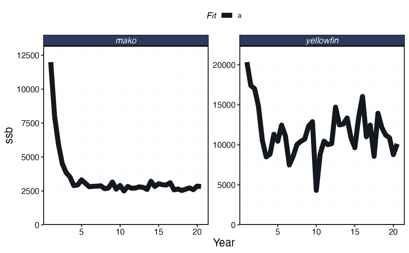

sim$fauna |>
  filter(age == min(age)) |>
  group_by(step, critter) |> 
  summarise(n = sum(n)) |> 
  ggplot(aes(step, n)) +
  geom_line() +
  geom_point() +
  facet_wrap(~critter, scales = "free_y") + 
  scale_y_continuous(limits = c(0, NA))
#> `summarise()` has grouped output by 'step'. You can override using the
#> `.groups` argument.

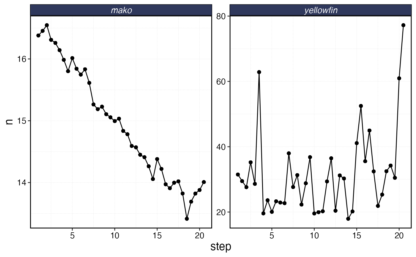
Timeline of recruits (age 0 fish) into the population over time given degrees of variation and autocorrelation in the recruitment process.

We can expand on this simple analysis by adding in a new feature, a correlation matrix for the recruitment deviates between the two simulated species. As this is a simple two-species system, this is just a two x two matrix with the off-diagonal elements indicating the correlation between the recruitment deviates of the two species. We will then pass this matrix to the simmar function.

critter_correlations <- matrix(c(1, -.8, -.8, 1), nrow = 2, byrow = TRUE)


# run simulations

a <- Sys.time()

recruitment_sim <- simmar(
  fauna = fauna,
  fleets = fleets,
  steps = steps,
  cor_rec = critter_correlations
)

Sys.time() - a
#> Time difference of 0.103061 secs

sim <- process_marlin(recruitment_sim)

sim$fauna |>
  filter(age == min(age)) |>
  select(step, patch, critter, n) |>
  group_by(critter, step) |> 
  summarise(n = sum(n)) |> 
  pivot_wider(names_from = critter, values_from = n) |>
  ggplot(aes(mako, yellowfin)) +
  geom_point()
#> `summarise()` has grouped output by 'critter'. You can override using the
#> `.groups` argument.

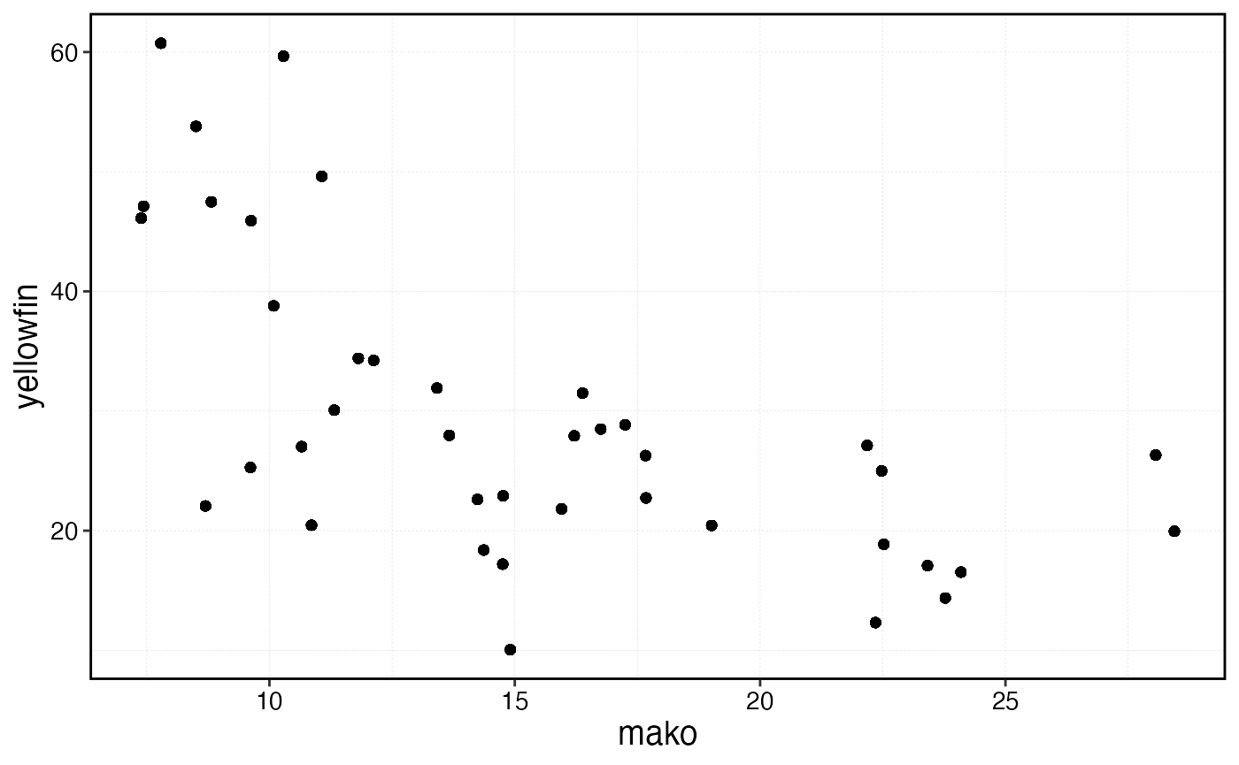
Scatter plot of negatively correlated recruitment between the two simulated species.

Users can also supply their own matrix of recruitment deviates. This matrix has number of columns equal to the number of critters, and rows equal to the number of years to be simulated plus one additional number of seasons per year (a required buffer). This step can be useful if for example the user wants to share the same vector of recruitment deviates across multiple simulations, or generate more complex recruitment deviates driven by for example environmental covariates.

sigma_recs <- purrr::map_dbl(fauna, "sigma_rec") # gather recruitment standard deviations

ac_recs <- purrr::map_dbl(fauna, "ac_rec") # gather autocorrelation in recruitment standard deviations

n_critters <- length(fauna)

covariance_rec <- critter_correlations * (sigma_recs %o% sigma_recs)

rec_steps <- steps + seasons

log_rec_devs <- matrix(NA, nrow = rec_steps, ncol = n_critters, dimnames = list(1:(rec_steps), names(fauna)))

log_rec_devs[1, ] <- mvtnorm::rmvnorm(1, rep(0, n_critters), sigma = covariance_rec)

for (i in 2:rec_steps) {
  log_rec_devs[i, ] <- ac_recs * log_rec_devs[i - 1, ] + sqrt(1 - ac_recs^2) * mvtnorm::rmvnorm(1, rep(0, n_critters), sigma = covariance_rec)
}

a <- Sys.time()

recruitment_sim <- simmar(
  fauna = fauna,
  fleets = fleets,
  steps = steps,
  log_rec_devs = log_rec_devs
)

Sys.time() - a
#> Time difference of 0.1133399 secs

sim <- process_marlin(recruitment_sim)

sim$fauna |>
  filter(age == min(age)) |>
  select(step, critter, n) |>
    group_by(critter, step) |> 
  summarise(n = sum(n)) |>
  pivot_wider(names_from = critter, values_from = n) |>
  ggplot(aes(mako, yellowfin)) +
  geom_point()
#> `summarise()` has grouped output by 'critter'. You can override using the
#> `.groups` argument.

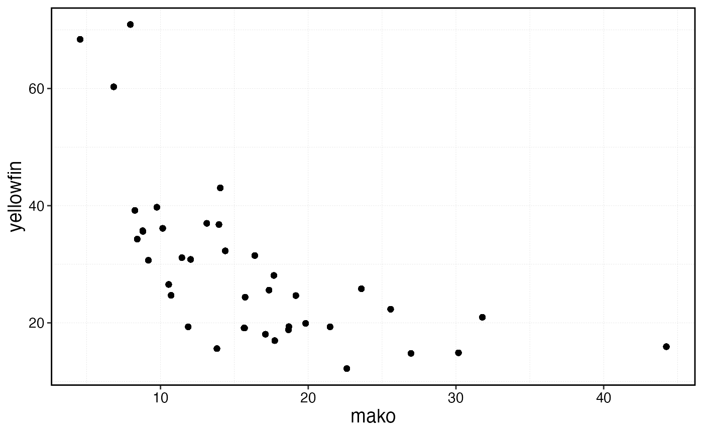
Scatter plot of externally supplied negatively correlated recruitment between the two simulated species.