Don't Be a Square

marlin defaults to a square resolution with equal numbers of cells in the X and Y directions for the simulation grid. But no need for you to get stuck in a square!

The resolution parameter allows you to specify any rectangular shape for your simulation space.

In the example below, we’ll simulate coastal rockfish species living along a west-facing coastline with a rapid dropoff to deep waters that the species does not live in.

In this case, we’ll use the resolution parameter to define a system that is 6 cells wide by 42 cells tall.

Each cell will have an area of 10km², meaning that the simulation area is 2,520 KM² and covers roughly 132 KM “north” to “south”

library(marlin)

library(tidyverse)

options(dplyr.summarise.inform = FALSE)

theme_set(marlin::theme_marlin(base_size = 14))

resolution <- c(10,100) #specify a 10 wide by 100 tall grid

patch_area <- 10 # 10km2

years <- 10

rockfish_diffusion <- 2 #KM2 / year

We’ll now make up a habitat layer in which the species prefers to live closter to shore (with shore being on the eastern edge of the simulation space)

coastal_habitat <- expand_grid(x = 1:resolution[1], y = 1:resolution[2]) %>%
  dplyr::mutate(habitat =  -.2 + .2 *x,
  habitat = habitat / max(habitat) * rockfish_diffusion) |> 
  pivot_wider(names_from = y, values_from = habitat) %>% 
  select(-x) %>% 
  as.matrix()

And from there we pass things to the usual sets of functions

fauna <- 
  list(
    "rockfish" = create_critter(
      common_name = "blue rockfish",
      adult_diffusion = 10,
      density_dependence = "post_dispersal",
      habitat = coastal_habitat,
      patch_area = patch_area,
      seasons = 4,
      fished_depletion = .25,
      resolution = resolution,
      steepness = 0.6,
      ssb0 = 42,
      m = 0.4
    ),
      "lingcod" = create_critter(
      common_name = "lingcod",
      adult_diffusion = 10,
      density_dependence = "post_dispersal",
      habitat = coastal_habitat,
      patch_area = patch_area,
      seasons = 4,
      fished_depletion = .7,
      resolution = resolution,
      steepness = 0.6,
      ssb0 = 100,
      m = 0.2
    )
  )


fleets <- list(
  "dayboats" = create_fleet(
    list("rockfish" = Metier$new(
        critter = fauna$rockfish,
        price = 10,
        sel_form = "logistic",
        sel_start = 1,
        sel_delta = .01,
        catchability = 0,
        p_explt = 1
      ),
      "lingcod" = Metier$new(
        critter = fauna$lingcod,
        price = 10,
        sel_form = "logistic",
        sel_start = 1,
        sel_delta = .01,
        catchability = 0,
        p_explt = 1
      )
    ),
    base_effort = prod(resolution),
    resolution = resolution
  )
)


fleets <- tune_fleets(fauna, fleets, tune_type = "depletion") 

start_time <- Sys.time()

coastline_sim <- simmar(fauna = fauna,
                  fleets = fleets,
                  years = years)

Sys.time() - start_time
#> Time difference of 1.166953 secs
  

processed_coastline <- process_marlin(coastline_sim, keep_age = FALSE)

plot_marlin(`Coastline Simulation` = processed_coastline, plot_type = "space")
#> Warning in plot_marlin(`Coastline Simulation` = processed_coastline, plot_type
#> = "space"): Can only plot one time step for spatial plots, defaulting to last
#> of the supplied steps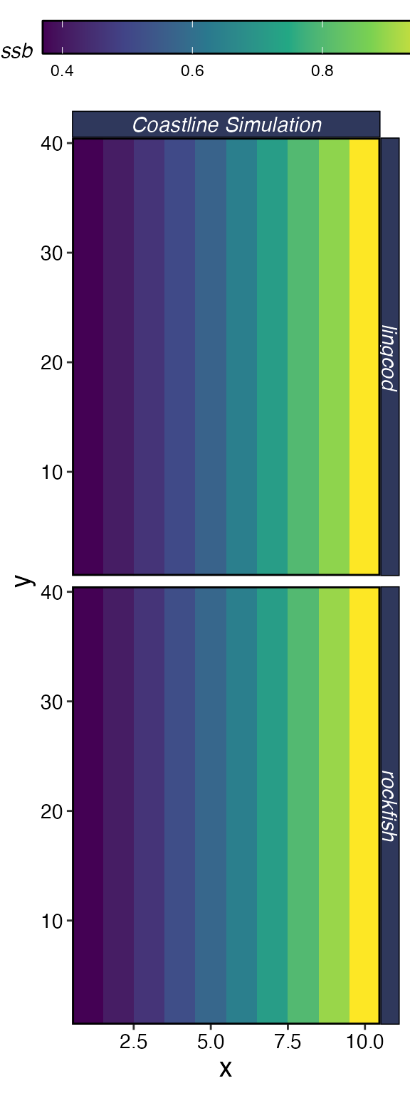

Rectangular simulation of a coastal rockfish species