Recruitment, Dispersal, and MPA Performance

Marine protected areas work by removing fishing mortality from a set of patches. But whether that local protection translates into population-wide benefits depends in part on recruitment: where new fish come from, how far larvae travel, and when density dependence kicks in relative to dispersal.

marlin implements five density dependence forms and allows independent control of recruit dispersal distance. This vignette isolates those mechanisms to show how they interact with MPA placement. The setup deliberately holds adult movement and habitat constant so that all spatial dynamics arise from the recruitment process.

Recruitment in marlin

All five recruitment forms in marlin are variants of the Beverton-Holt spawner-recruit relationship, parameterized around steepness ($h$). Steepness controls how sensitive recruitment is to spawning biomass: when $h = 1$ recruitment is independent of SSB, and as $h$ approaches 0.2 recruitment becomes a linear function of SSB. The forms differ in where density dependence acts (globally vs locally), when it acts relative to larval dispersal, and how recruits are distributed across patches. Following Babcock and MacCall (2011), we denote $r0_p$ as the unfished recruitment in patch $p$, $\text{SSB}_{t,p}$ as spawning biomass in patch $p$ at time $t$, $\text{SSB0}_p$ as unfished spawning biomass in patch $p$, and $\epsilon_t$ as a log-normal recruitment deviate. $\mathbf{d}^l$ is the recruit movement (dispersal) matrix derived from recruit_home_range.

1. Global Habitat (global_habitat)

Density dependence operates on the total SSB summed across all patches. The resulting recruits are then distributed among patches in proportion to recruitment habitat quality ($r0_p / \sum_p r0_p$):

$$N_{t,p,a=1} = \left( \frac{0.8 \times \sum_p r0_p \times h \times \sum_p \text{SSB}_{t-1,p}}{0.2 \times \sum_p \text{SSB0}_p \times (1 - h) + (h - 0.2) \times \sum_p \text{SSB}_{t-1,p}} \right) \times \frac{r0_p}{\sum_p r0_p} \times \epsilon_t$$

This form treats the entire domain as a single stock for the purposes of the stock-recruit relationship. The spatial distribution of recruits is determined entirely by habitat quality, not by where the spawners are. Larval dispersal (recruit_home_range) has no effect because recruit placement is set by habitat. This is appropriate when larval connectivity is so high that the population is effectively a single reproductive unit, and settlement patterns are driven by habitat suitability rather than proximity to spawners.

2. Local Habitat (local_habitat)

Each patch has its own independent stock-recruit relationship. Density dependence is purely local, and recruits remain in the patch where they were produced:

$$N_{t,p,a=1} = \left( \frac{0.8 \times r0_p \times h \times \text{SSB}_{t-1,p}}{0.2 \times \text{SSB0}_p \times (1 - h) + (h - 0.2) \times \text{SSB}_{t-1,p}} \right) \times \epsilon_t$$

This is the most spatially conservative form: what happens in a patch stays in that patch. Each patch’s carrying capacity is set by its own $r0_p$ and $\text{SSB0}_p$. As with global_habitat, recruit_home_range does not affect the spatial distribution of recruits because they are assigned to their home patch. This form is appropriate for sedentary species with limited larval dispersal where local density dependence is strong.

3. Pre-Dispersal (pre_dispersal)

Density-dependent competition occurs locally in the spawning patch, and then surviving recruits disperse according to the recruit movement matrix $\mathbf{d}^l$:

$$N_{t,p,a=1} = \left( \frac{0.8 \times r0_p \times h \times \text{SSB}_{t-1,p}}{0.2 \times \text{SSB0}_p \times (1 - h) + (h - 0.2) \times \text{SSB}_{t-1,p}} \right) \times \mathbf{d}^l \times \epsilon_t$$

The competitive bottleneck is set by conditions at the origin patch. This matters for MPAs: a protected patch with high SSB produces recruits that survive the local density-dependent filter and then spread to neighboring (potentially fished) patches. In the case of an MPA acting as a larval source. recruit_home_range directly controls how far that subsidy reaches — short dispersal keeps benefits local, long dispersal spreads them across the domain. This timing of density dependence might be appropriate for spawning aggregations where density dependence happens as a result of predator aggregations on large spawning events.

4. Post-Dispersal (post_dispersal)

Larvae disperse first according to $\mathbf{d}^l$, and then density-dependent recruitment occurs at the destination patch based on the local SSB there:

$$\text{larv}_{t,p} = \text{SSB}_{t-1,p} \times \mathbf{d}^l$$

$$N_{t,p,a=1} = \left( \frac{0.8 \times r0_p \times h \times \text{larv}_{t,p}}{0.2 \times \text{SSB0}_p \times (1 - h) + (h - 0.2) \times \text{larv}_{t,p}} \right) \times \epsilon_t$$

The key distinction from pre-dispersal: competition is based on SSB at the settlement site, not the origin. Larvae from a protected MPA patch disperse outward, but when they arrive at a fished (lower-SSB) destination they face the same density-dependent environment as locally-produced recruits. This could be a scenario where the key bottleneck in recruitment is available habitat at the time of settlement.

5. Global SSB (global_ssb)

Like global_habitat, density dependence operates on total SSB across all patches. But instead of distributing recruits by habitat quality, recruits are allocated in proportion to the spatial distribution of SSB:

$$N_{t,p,a=1} = \left( \frac{0.8 \times \sum_p r0_p \times h \times \sum_p \text{SSB}_{t-1,p}}{0.2 \times \sum_p \text{SSB0}_p \times (1 - h) + (h - 0.2) \times \sum_p \text{SSB}_{t-1,p}} \right) \times \frac{\text{SSB}_{t-1,p}}{\sum_p \text{SSB}_{t-1,p}} \times \epsilon_t$$

This creates a positive feedback: patches with more SSB receive more recruits, which builds more SSB. An MPA amplifies this loop by maintaining high local SSB, attracting a disproportionate share of the system-wide recruitment. As with global_habitat, recruit_home_range does not affect the spatial allocation of recruits because placement is determined by the SSB distribution.

Recruitment deviates

Log-normal recruitment deviates $\epsilon_t$ are generated with optional autocorrelation:

$$\upsilon_t \sim \begin{cases} N(0, \sigma_r) & \text{if } t = 1 \\ \rho \log(\upsilon_{t-1}) + \sqrt{1 - \rho^2} \, N(0, \sigma_r) & \text{if } t > 1 \end{cases}$$

where $\sigma_r$ is sigma_rec and $\rho$ is ac_rec. Raw deviates are converted with a bias correction to ensure the mean recruitment is unbiased in arithmetic space. See the Working with Recruitment Deviates vignette for more detail on controlling stochastic recruitment.

Vignette Overview

With the recruitment equations in hand, we now demonstrate how these five forms interact with MPA placement and larval dispersal distance. We will:

1. Build a system with uniform adult habitat but heterogeneous recruitment habitat
2. Fish the population to 25% of unfished biomass
3. Place an MPA over the best recruitment habitat
4. Track patch-level recovery under all five density dependence forms and three levels of recruit dispersal

library(marlin)
library(tidyverse)
library(patchwork)

theme_set(marlin::theme_marlin(base_size = 12))

Setting Up the Seascape

We use a 10×10 grid with 10 km² patches (each patch is ~3.2 km on a side, total domain ~32 × 32 km).

Adult habitat is uniform everywhere: adults have no spatial preference and low home range, so they essentially stay where they are. This isolates the recruitment channel.

Recruitment habitat is spatially structured, generated by sim_habitat with kp = 0.01 for broad, smooth gradients. This creates a clear “good nursery” region and a “poor nursery” region.

resolution <- c(10, 10)
patch_area <- 10  # km^2 per patch
years <- 50
mpa_year <- 25    # MPA introduced halfway through
seasons <- 1
time_step <- 1 / seasons

# Uniform adult habitat: no spatial preference for adults
adult_habitat <- matrix(1, nrow = resolution[2], ncol = resolution[1])

# Heterogeneous recruitment habitat
recruit_hab <- sim_habitat(
  "species",
  kp = 0.01,
  resolution = resolution,
  patch_area = patch_area,
  output = "list"
)
recruit_habitat <- recruit_hab$critter_distributions$species

expand_grid(x = 1:resolution[1], y = 1:resolution[2]) |>
  mutate(recruit_habitat = as.vector(recruit_habitat)) |>
  ggplot(aes(x, y, fill = recruit_habitat)) +
  geom_tile() +
  scale_fill_viridis_c(name = "Recruit\nhabitat") +
  coord_equal() +
  labs(title = "Recruitment Habitat Quality")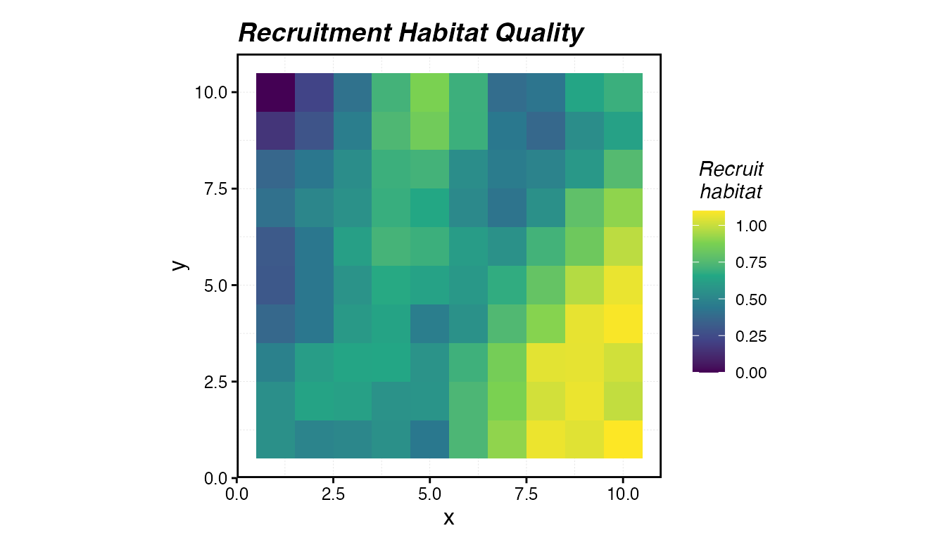

Recruitment habitat quality across the seascape. Brighter colours indicate better nursery conditions.

Designing the MPA

We protect the top 30% of patches ranked by recruitment habitat quality. This represents an MPA placed deliberately over the best nursery grounds, a common strategy in spatial planning.

patches <- expand_grid(x = 1:resolution[1], y = 1:resolution[2]) |>
  mutate(
    patch = row_number(),
    r_hab = as.vector(recruit_habitat)
  )

mpa_threshold <- quantile(patches$r_hab, 0.7)

mpa_locations <- patches |>
  mutate(mpa = r_hab >= mpa_threshold)

ggplot(mpa_locations, aes(x, y)) +
  geom_tile(aes(fill = r_hab)) +
  geom_tile(
    data = filter(mpa_locations, mpa),
    aes(x, y),
    fill = NA, color = "cyan", linewidth = 0.8
  ) +
  scale_fill_viridis_c(name = "Recruit\nhabitat") +
  coord_equal() +
  labs(title = "MPA Placement (outlined) on Recruitment Habitat")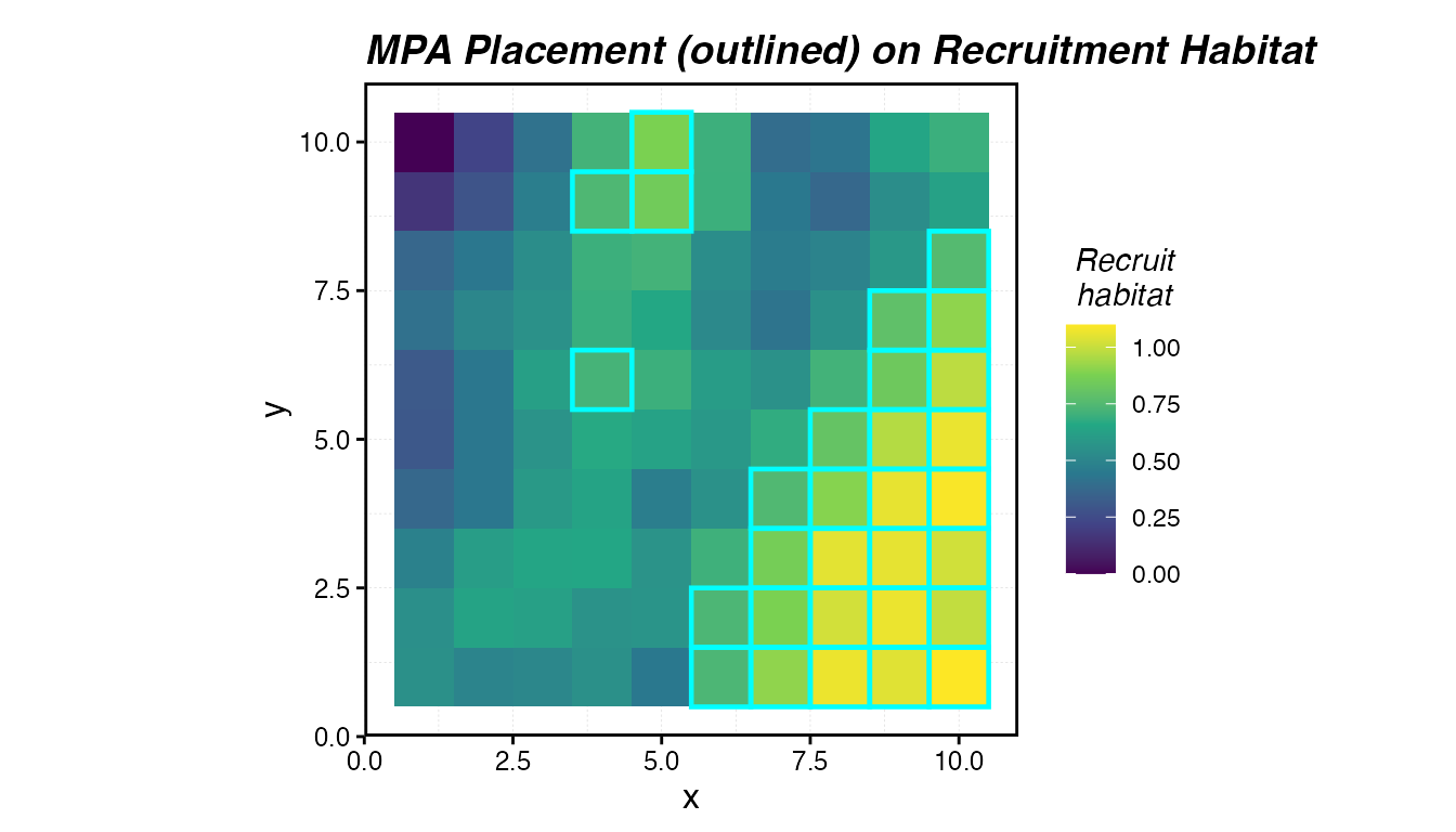

MPA placement (teal) targeting the highest-quality recruitment habitat.

The Scenario Grid

We cross all five density dependence forms with three recruit dispersal distances:

• recruit_home_range = 2: larvae settle within ~2 km (less than one patch width). Recruitment is essentially local.
• recruit_home_range = 10: larvae disperse ~10 km (~3 patches). Regional connectivity.
• recruit_home_range = 100: larvae spread across the entire domain. Recruitment is effectively global.

dd_forms <- c(
  "global_habitat",
  "local_habitat",
  "pre_dispersal",
  "post_dispersal",
  "global_ssb"
)

recruit_ranges <- c(2, 10, 100)

scenarios <- expand_grid(
  dd = dd_forms,
  recruit_home_range = recruit_ranges
) |>
  mutate(scenario_id = row_number())

scenarios
#> # A tibble: 15 × 3
#>    dd             recruit_home_range scenario_id
#>    <chr>                       <dbl>       <int>
#>  1 global_habitat                  2           1
#>  2 global_habitat                 10           2
#>  3 global_habitat                100           3
#>  4 local_habitat                   2           4
#>  5 local_habitat                  10           5
#>  6 local_habitat                 100           6
#>  7 pre_dispersal                   2           7
#>  8 pre_dispersal                  10           8
#>  9 pre_dispersal                 100           9
#> 10 post_dispersal                  2          10
#> 11 post_dispersal                 10          11
#> 12 post_dispersal                100          12
#> 13 global_ssb                      2          13
#> 14 global_ssb                     10          14
#> 15 global_ssb                    100          15

Running the Scenarios

Each scenario creates a fresh critter, tunes the fleet to achieve 25% depletion, then runs a 50-year simulation with the MPA introduced at year 25. We use sigma_rec = 0 to eliminate stochastic noise and isolate the structural effects of density dependence and dispersal.

run_scenario <- function(dd, recruit_home_range, scenario_id, ...) {

  fauna <- list(
    "species" = create_critter(
      common_name = "bigeye tuna",
      habitat = list(adult_habitat),
      season_blocks = list(1),
      recruit_habitat = recruit_habitat,
      adult_home_range = 1,
      recruit_home_range = recruit_home_range,
      density_dependence = dd,
      fished_depletion = 0.25,
      seasons = seasons,
      resolution = resolution,
      patch_area = patch_area,
      steepness = 0.6,
      ssb0 = 1000,
      sigma_rec = 0
    )
  )

  fleets <- list(
    "fleet" = create_fleet(
      list(
        "species" = Metier$new(
          critter = fauna$species,
          price = 10,
          sel_form = "logistic",
          sel_start = 1,
          sel_delta = 0.01,
          catchability = 0,
          p_explt = 1
        )
      ),
      base_effort = prod(resolution),
      resolution = resolution,
      fleet_model = "constant_effort"
    )
  )

  fleets <- tune_fleets(fauna, fleets, tune_type = "depletion")

  sim <- simmar(
    fauna = fauna,
    fleets = fleets,
    years = years,
    manager = list(
      mpas = list(
        locations = mpa_locations,
        mpa_year = mpa_year
      )
    )
  )

  proc <- process_marlin(sim, time_step = time_step)

  # Tag results with scenario metadata
  proc$fauna <- proc$fauna |>
    mutate(
      dd = dd,
      recruit_home_range = recruit_home_range,
      scenario_id = scenario_id
    )

  proc$fleets <- proc$fleets |>
    mutate(
      dd = dd,
      recruit_home_range = recruit_home_range,
      scenario_id = scenario_id
    )

  proc
}

results <- pmap(scenarios, run_scenario)

Assembling Results

We combine all scenario outputs and classify each patch as inside or outside the MPA.

all_fauna <- map_dfr(results, ~ .x$fauna)

all_fleets <- map_dfr(results, ~ .x$fleets)

# Add MPA status to each patch
all_fauna <- all_fauna |>
  left_join(
    mpa_locations |> select(x, y, mpa),
    by = c("x", "y")
  )

# Nice labels for plotting
dd_labels <- c(
  "global_habitat"  = "Global Habitat",
  "local_habitat"   = "Local Habitat",
  "pre_dispersal"   = "Pre-dispersal",
  "post_dispersal"  = "Post-dispersal",
  "global_ssb"      = "Global SSB"
)

rhr_labels <- c(
  "2"   = "Local (2 km)",
  "10"  = "Regional (10 km)",
  "100" = "Global (100 km)"
)

all_fauna <- all_fauna |>
  mutate(
    dd_label = factor(dd_labels[dd], levels = dd_labels),
    rhr_label = factor(
      rhr_labels[as.character(recruit_home_range)],
      levels = rhr_labels
    ),
    mpa_status = if_else(mpa, "Inside MPA", "Outside MPA")
  )

How Does SSB Recover?

The first key question: after the MPA is implemented, does biomass rebuild inside the MPA, and does any of that benefit spill over to fished areas?

We plot mean SSB (summed across ages) per patch over time, split by MPA status.

ssb_time <- all_fauna |>
  group_by(dd_label, rhr_label, mpa_status, x, y, step) |>
  summarise(ssb = sum(ssb, na.rm = TRUE), .groups = "drop") |>
  group_by(dd_label, rhr_label, mpa_status, step) |>
  summarise(
    mean_ssb = mean(ssb, na.rm = TRUE),
    .groups = "drop"
  )

ggplot(ssb_time, aes(step, mean_ssb, color = mpa_status)) +
  geom_line(linewidth = 0.7) +
  geom_vline(xintercept = mpa_year, linetype = "dashed", color = "grey40") +
  facet_grid(dd_label ~ rhr_label, scales = "free_y") +
  scale_color_manual(
    values = c("Inside MPA" = "#1b9e77", "Outside MPA" = "#d95f02"),
    name = NULL
  ) +
  labs(
    x = "Year",
    y = "Mean SSB per patch",
    title = "Biomass Recovery Inside vs. Outside the MPA"
  ) +
  theme(legend.position = "bottom")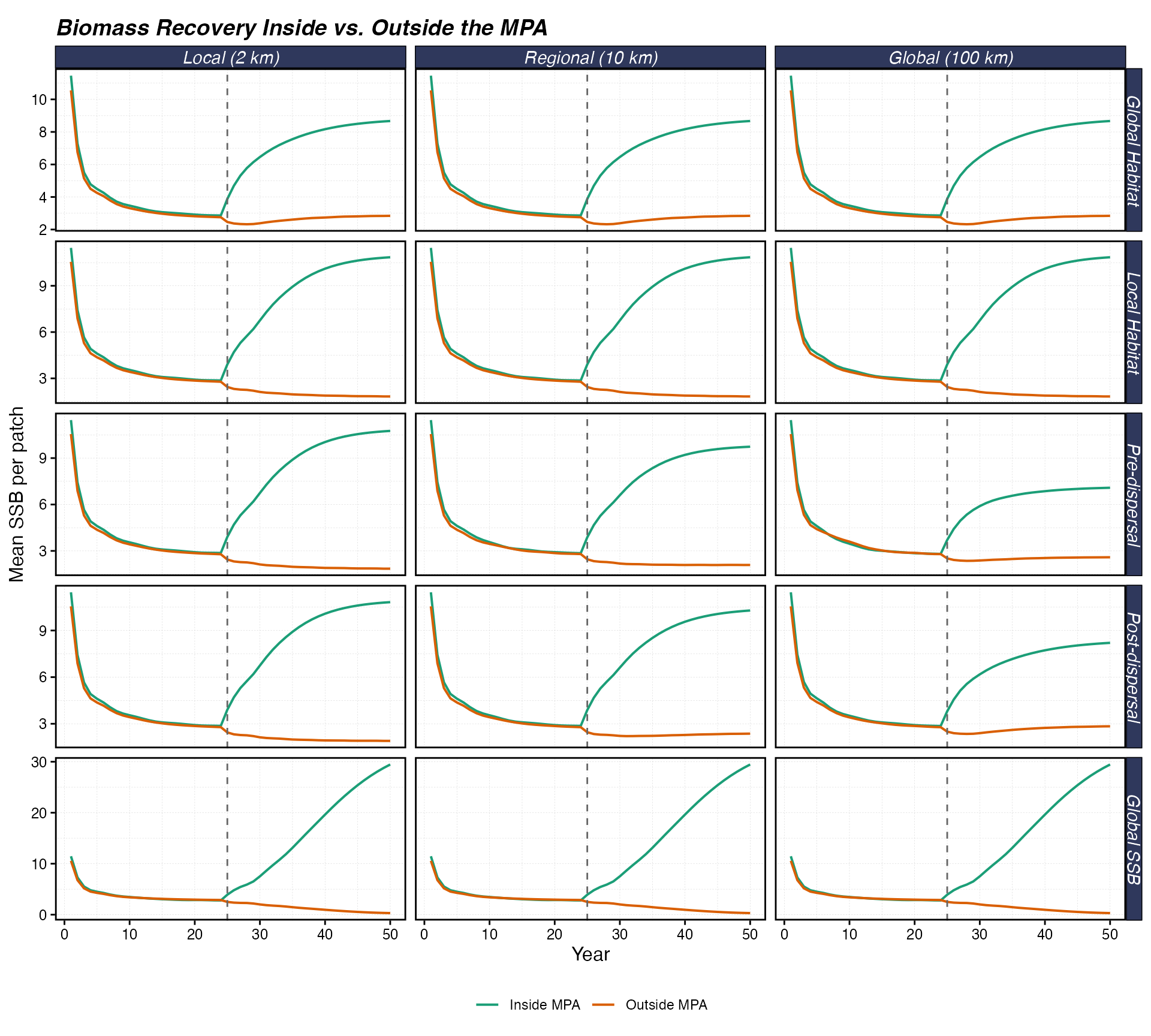

Mean SSB per patch over time, inside vs. outside the MPA. The vertical dashed line marks MPA implementation at year 25. Rows show density dependence forms; columns show recruit dispersal distance.

Total Population Response

The MPA protects local biomass, but does the overall population benefit? This depends on whether the MPA creates a net recruitment subsidy (spillover via larvae) or simply redistributes existing production.

total_ssb <- all_fauna |>
  group_by(dd_label, rhr_label, x, y, step) |>
  summarise(ssb = sum(ssb, na.rm = TRUE), .groups = "drop") |>
  group_by(dd_label, rhr_label, step) |>
  summarise(total_ssb = sum(ssb, na.rm = TRUE), .groups = "drop")

ggplot(total_ssb, aes(step, total_ssb, color = rhr_label)) +
  geom_line(linewidth = 0.7) +
  geom_vline(xintercept = mpa_year, linetype = "dashed", color = "grey40") +
  facet_wrap(~dd_label, scales = "free_y", ncol = 5) +
  scale_color_brewer(palette = "Set1", name = "Recruit dispersal") +
  labs(
    x = "Year",
    y = "Total SSB (all patches)",
    title = "Total Population Biomass by Density Dependence Form"
  ) +
  theme(legend.position = "bottom")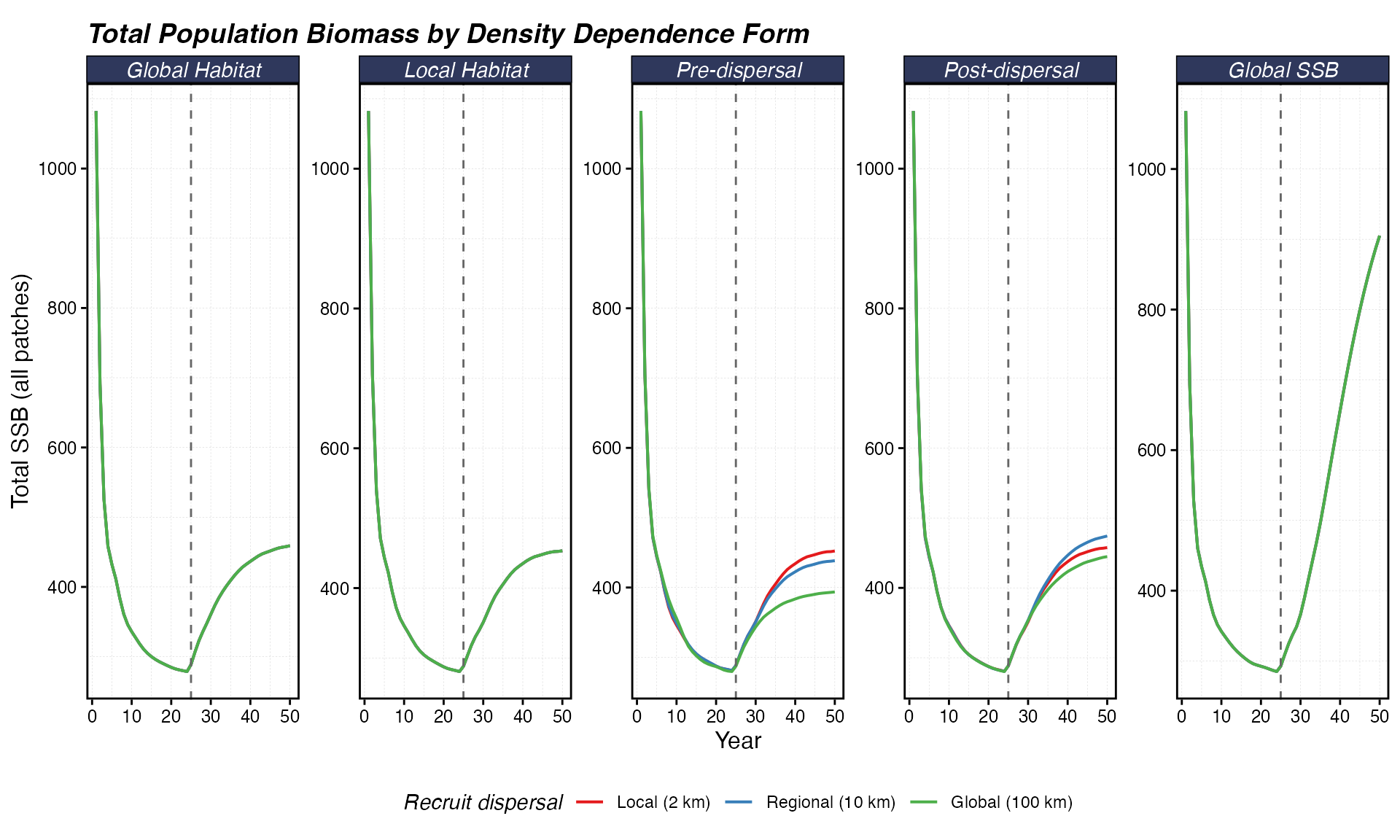

Total SSB across the entire domain over time. A rising trajectory after year 25 indicates the MPA produces a net population benefit; a flat line means only redistribution.

Spatial Biomass Patterns at the End

Spatial maps of biomass at the final time step reveal where fish accumulate and whether the MPA creates biomass gradients (“fishing the line” effects).

final_step <- max(all_fauna$step)

spatial_final <- all_fauna |>
  filter(step == final_step) |>
  group_by(dd_label, rhr_label, x, y, mpa) |>
  summarise(ssb = sum(ssb, na.rm = TRUE), .groups = "drop")

ggplot(spatial_final, aes(x, y, fill = ssb)) +
  geom_tile() +
  geom_tile(
    data = filter(spatial_final, mpa),
    fill = NA, color = "cyan", linewidth = 0.4
  ) +
  facet_grid(dd_label ~ rhr_label) +
  scale_fill_viridis_c(name = "SSB") +
  coord_equal() +
  labs(title = "Spatial SSB at Final Time Step") +
  theme(axis.text = element_blank(), axis.ticks = element_blank())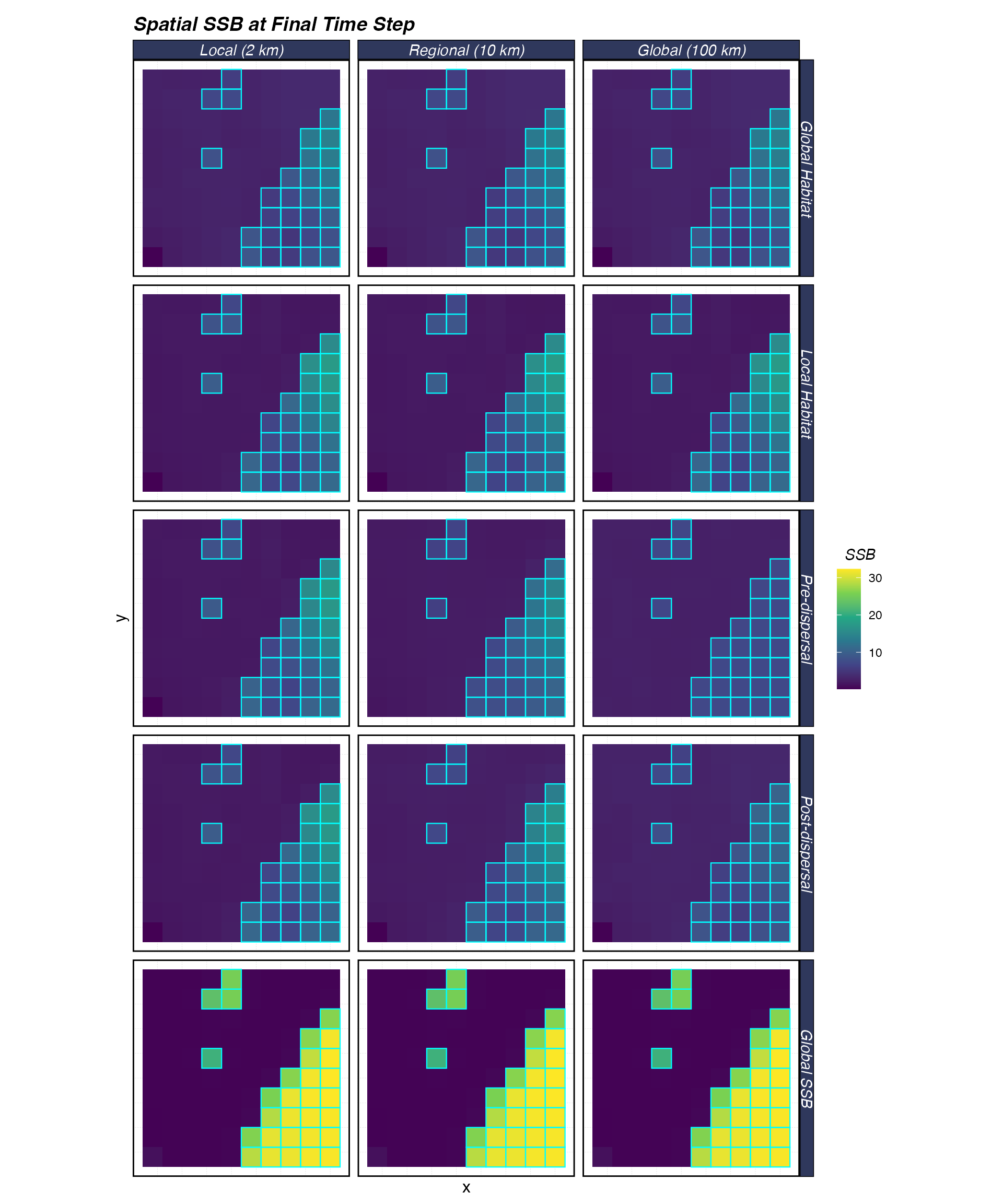

Spatial distribution of SSB at the final time step. Cyan outlines show MPA boundaries. Rows = density dependence; columns = recruit dispersal distance.

The MPA “Multiplier”: Inside vs. Outside

A useful summary statistic is the ratio of mean SSB inside the MPA to mean SSB outside, computed at the final time step. Ratios greater than 1 indicate biomass accumulation inside the reserve; values near 1 suggest benefits have been exported.

response_ratio <- spatial_final |>
  group_by(dd_label, rhr_label, mpa) |>
  summarise(mean_ssb = mean(ssb), .groups = "drop") |>
  pivot_wider(names_from = mpa, values_from = mean_ssb) |>
  mutate(ratio = `TRUE` / `FALSE`)

ggplot(response_ratio, aes(rhr_label, ratio, fill = dd_label)) +
  geom_col(position = position_dodge(width = 0.8), width = 0.7) +
  geom_hline(yintercept = 1, linetype = "dashed") +
  scale_fill_brewer(palette = "Set2", name = "Density\ndependence") +
  labs(
    x = "Recruit Dispersal Distance",
    y = "Response Ratio (Inside / Outside)",
    title = "MPA Response Ratio by Scenario"
  ) +
  theme(legend.position = "right")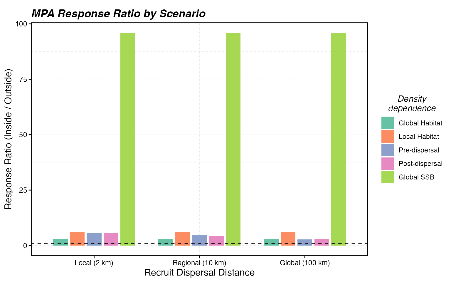

Response ratio (mean SSB inside MPA / mean SSB outside MPA) at the final time step. Higher values indicate stronger local accumulation; values near 1 suggest exported benefits.

Catch Impacts

MPAs displace fishing effort. How much catch is lost, and does it depend on how recruitment works?

total_catch <- all_fauna |>
  group_by(dd_label, rhr_label, x, y, step) |>
  summarise(catch = sum(c, na.rm = TRUE), .groups = "drop") |>
  group_by(dd_label, rhr_label, step) |>
  summarise(total_catch = sum(catch, na.rm = TRUE), .groups = "drop")

ggplot(total_catch, aes(step, total_catch, color = rhr_label)) +
  geom_line(linewidth = 0.7) +
  geom_vline(xintercept = mpa_year, linetype = "dashed", color = "grey40") +
  facet_wrap(~dd_label, scales = "free_y", ncol = 5) +
  scale_color_brewer(palette = "Set1", name = "Recruit dispersal") +
  labs(
    x = "Year",
    y = "Total Catch",
    title = "Catch Trajectories by Scenario"
  ) +
  theme(legend.position = "bottom")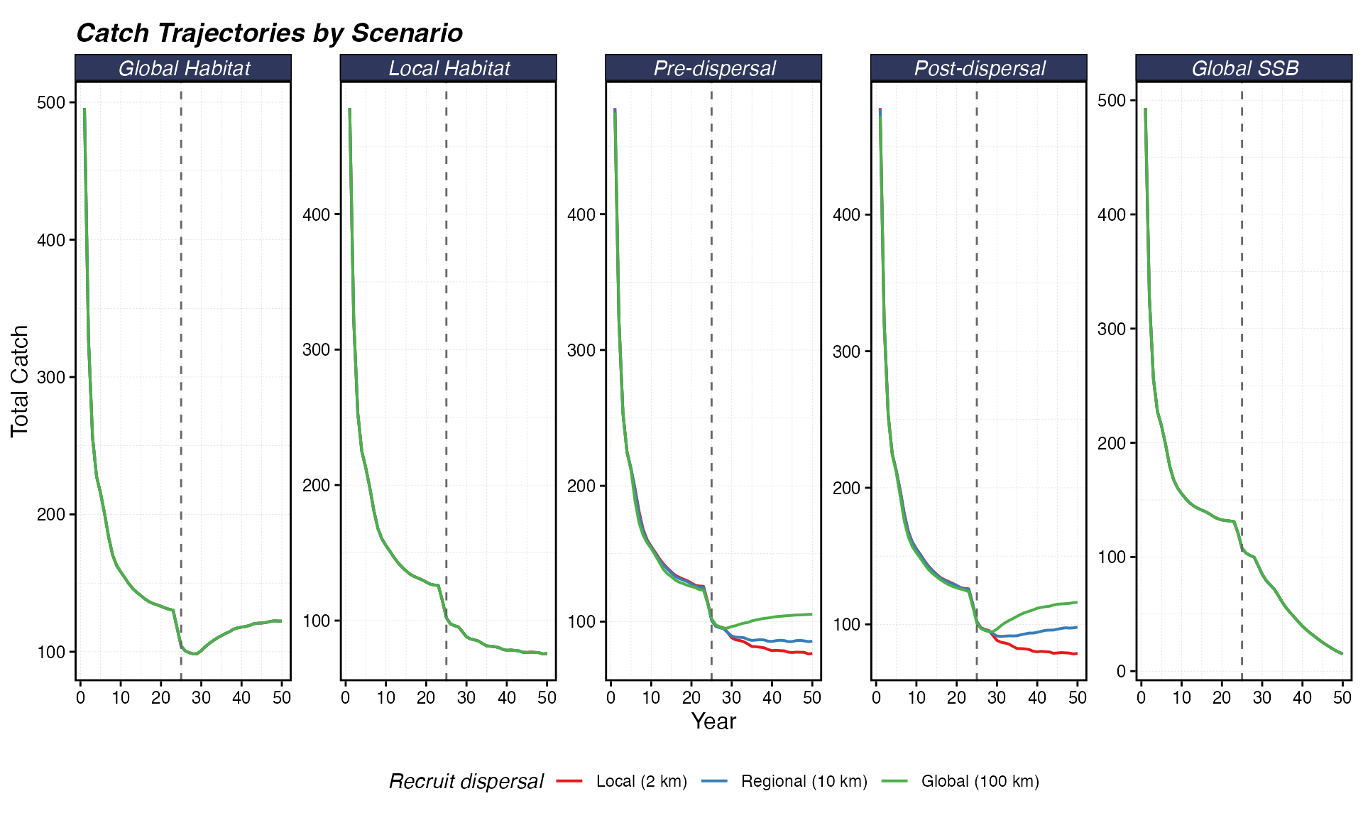

Total catch over time by scenario. The dashed line marks MPA implementation. Catch may decline initially as effort is displaced from productive patches, then partially recover as biomass rebuilds.

Next Steps

This vignette focused on recruitment mechanics in isolation. In reality, adult movement, fleet redistribution, and habitat heterogeneity all interact with these dynamics. See:

• Setting & Understanding Movement Rates for adult movement
• Measure MPA Gradients for quantifying spillover from adult movement
• Spatial Allocation Strategies for how fleets respond to MPAs
• Getting Started for a full walkthrough combining all components