Spatial Allocation Memory • marlin

The spatial-allocation vignette covers what each spatial_allocation strategy does. This companion focuses on the memory_halflife argument to create_fleet(): when it matters, what it fixes, and what its failure mode looks like.

By default the objective surface a fleet acts on is rebuilt fresh each step from the previous step’s outcomes — a one-step-lag signal. Under strong fleet-biomass coupling this can drive period-2 sawtooth oscillation in patch effort: last-step buffet picks where to fish, this-step fishing changes biomass, next-step buffet inverts. memory_halflife > 0 replaces the raw per-patch objective $O_p$ with an exponentially-smoothed version: a weighted average in which the weight on the observation from $k$ steps ago decays geometrically, so the most recent observation has the largest influence and older ones fade away:

$\tilde{O}_p^{(t)} = \alpha \, O_p^{(t)} + (1 - \alpha) \, \tilde{O}_p^{(t-1)}, \qquad \alpha = 1 - 0.5^{1 / h_{\text{steps}}}$

The half-life is specified in years and converted internally to steps ( $h_{\text{steps}} = h_{\text{years}} \times \text{steps\_per\_year}$ ), so the same value produces the same calendar-time smoothing regardless of seasons per year. Three implementation details matter:

Closed-patch policy is “freeze and resume”: the smoothed surface only updates on currently-open patches. Closed patches retain their last-seen smoothed value, so an MPA that closes then re-opens a patch sees the fleet’s pre-closure memory of it.
Warm-up ramp: on the very first step the smoothed history is seeded with the observed objective surface. For the next few steps the effective smoothing weight is $\alpha_{\text{eff}} = \max(\alpha, 1/n)$ , where $n$ counts updates since the seed step — so the smoothed surface behaves like a running mean over the warm-up window rather than being anchored to the seed value. Once $1/n$ drops below the asymptotic $\alpha$ , the ramp is done.
Phase-lag tradeoff: exponential smoothing introduces a phase lag of roughly $1.44 \times h_{\text{years}}$ years between a real change in patch marginal value and the fleet’s perceived value. Long half-lives can therefore replace high-frequency sawtooth with low-frequency overshoot — a different pathology.

Memory smooths only the spatial allocation objective. Total fleet effort under open_access or sole_owner still responds to the raw fleet-level profitability signal, which has its own slow timescale built in via the entry/exit caps.

Setup

We reuse the two-species, two-fleet, two-port system from the main spatial-allocation vignette, then build a marginal_profit allocator on both fleets — the configuration most prone to sawtooth — and close an offshore corner mid-run to force redistribution.

library(marlin)
library(ggplot2)
library(dplyr)
library(tidyr)

theme_set(marlin::theme_marlin(base_size = 12) +
            theme(legend.position = "top"))

resolution <- c(20, 20)
patches <- prod(resolution)
seasons <- 2
time_step <- 1 / seasons

ports <- data.frame(x = c(1, 8), y = c(1, 9))

critter_correlations <- matrix(c(1, -0.5,
                                 -0.5, 1), nrow = 2)

habitats <- sim_habitat(
  critters = c("bigeye", "skipjack"),
  kp = 0.1,
  critter_correlations = critter_correlations,
  resolution = resolution,
  patch_area = 1,
  output = "list"
)

bigeye_habitat <- habitats$critter_distributions$bigeye
skipjack_habitat <- habitats$critter_distributions$skipjack

fauna <-
  list(
    "bigeye" = create_critter(
      common_name = "bigeye tuna",
      habitat = list(bigeye_habitat),
      season_blocks = list(1:seasons),
      adult_home_range = 5,
      recruit_home_range = 10,
      density_dependence = "local_habitat",
      seasons = seasons,
      depletion = 0.5,
      init_explt = 0.2,
      explt_type = "f",
      resolution = resolution,
      steepness = 0.6,
      ssb0 = 1000
    ),
    "skipjack" = create_critter(
      scientific_name = "Katsuwonus pelamis",
      habitat = list(skipjack_habitat),
      season_blocks = list(1:seasons),
      adult_home_range = 3,
      recruit_home_range = 8,
      density_dependence = "local_habitat",
      seasons = seasons,
      depletion = 0.6,
      init_explt = 0.15,
      explt_type = "f",
      resolution = resolution,
      steepness = 0.7,
      ssb0 = 800
    )
  )

The fleet builder takes halflife and applies it to both fleets; the metier and port structure is identical to the main vignette.

build_fleets <- function(halflife,
                         spatial_allocation = "marginal_profit",
                         fleet_model = "constant_effort") {
  fleets <- list(
    "longline" = create_fleet(
      list(
        "bigeye" = Metier$new(
          critter = fauna$bigeye, price = 10,
          sel_form = "logistic", sel_start = 1, sel_delta = 0.01,
          catchability = 0, p_explt = 2
        ),
        "skipjack" = Metier$new(
          critter = fauna$skipjack, price = 5,
          sel_form = "logistic", sel_start = 0.8, sel_delta = 0.1,
          catchability = 0, p_explt = 1
        )
      ),
      ports = ports, base_effort = patches, resolution = resolution,
      spatial_allocation = spatial_allocation,
      fleet_model = fleet_model,
      cr_ratio = 1, travel_fraction = 0.7,
      memory_halflife = halflife,
      responsiveness = 0.025
    ),
    "handline" = create_fleet(
      list(
        "bigeye" = Metier$new(
          critter = fauna$bigeye, price = 10,
          sel_form = "logistic", sel_start = 1.2, sel_delta = 0.1,
          catchability = 0, p_explt = 1
        ),
        "skipjack" = Metier$new(
          critter = fauna$skipjack, price = 8,
          sel_form = "logistic", sel_start = 0.5, sel_delta = 0.2,
          catchability = 0, p_explt = 2
        )
      ),
      ports = ports, base_effort = patches, resolution = resolution,
      spatial_allocation = spatial_allocation,
      fleet_model = fleet_model,
      cr_ratio = 1, travel_fraction = 0.5,
      memory_halflife = halflife,
      responsiveness = 0.025
    )
  )
  tune_fleets(fauna, fleets, tune_type = "depletion")
}

Halflife sweep with an MPA closure

We close an offshore corner at year 8 and sweep memory_halflife across c(0, 1, 2) years. The expectation: at memory_halflife = 0 (legacy behaviour) the dynamics show visible high-frequency wiggle in individual patches; modest memory dampens it cleanly; very long memory introduces a different problem — low-frequency overshoot driven by the phase lag the smoothing imposes.

years_5    <- 20
mpa_year_5 <- 8

mpa_locs_5 <- expand_grid(x = 1:resolution[1], y = 1:resolution[2]) %>%
  mutate(mpa = x >= 12 & y >= 12)
manager_5 <- list(mpas = list(locations = mpa_locs_5, mpa_year = mpa_year_5))

halflives_5 <- c(0, 1, 2)

runs_5 <- lapply(halflives_5, function(hl) {
  sim  <- simmar(fauna = fauna, fleets = build_fleets(hl),
                 years = years_5, manager = manager_5)
  proc <- process_marlin(sim, time_step = time_step)
  list(halflife = hl, proc = proc)
})

Two patch-level metrics, computed on the post-MPA window:

lag-1 autocorrelation of patch effort (low / negative ⇒ sawtooth)
step-difference CV: sd(diff(effort)) / mean(effort), capturing high-frequency wiggle on top of any trend

post_mpa_metrics <- function(r, burn_after_mpa_years = 2) {
  start_step <- (mpa_year_5 + burn_after_mpa_years) * seasons
  r$proc$fleets %>%
    filter(step > start_step) %>%
    arrange(fleet, patch, step) %>%
    group_by(fleet, patch) %>%
    summarise(
      mean_effort  = mean(effort, na.rm = TRUE),
      effort_acf1  = if (n() > 3 && stats::sd(effort, na.rm = TRUE) > 0)
        stats::acf(effort, plot = FALSE, lag.max = 1)$acf[2] else NA_real_,
      step_diff_cv = if (n() > 3 && mean(effort, na.rm = TRUE) > 1e-9)
        stats::sd(diff(effort), na.rm = TRUE) / mean(effort, na.rm = TRUE) else NA_real_,
      .groups = "drop"
    ) %>%
    mutate(halflife = r$halflife)
}

all_metrics <- purrr::map_dfr(runs_5, post_mpa_metrics) %>%
  filter(mean_effort > 1e-3)

all_metrics %>%
  group_by(halflife, fleet) %>%
  summarise(
    n_patches            = n(),
    median_effort_acf1   = signif(median(effort_acf1, na.rm = TRUE), 3),
    median_step_diff_cv  = signif(median(step_diff_cv, na.rm = TRUE), 3),
    p90_step_diff_cv     = signif(quantile(step_diff_cv, 0.9, na.rm = TRUE), 3),
    .groups = "drop"
  ) %>%
  knitr::kable(digits = 3,
               caption = "Post-MPA per-patch effort autocorrelation and high-frequency wiggle, by halflife and fleet.")

Post-MPA per-patch effort autocorrelation and high-frequency wiggle, by halflife and fleet.
halflife	fleet	n_patches	median_effort_acf1
0	handline	319	NA
0	longline	319	NA
1	handline	319	NA
1	longline	319	NA
2	handline	319	NA
2	longline	319	NA

# Pick the 3 most-oscillating patches per fleet under the lowest halflife;
# trace each across all three runs.
baseline_hl  <- min(halflives_5)
top_patches  <- all_metrics %>%
  filter(halflife == baseline_hl) %>%
  group_by(fleet) %>%
  slice_max(step_diff_cv, n = 3, with_ties = FALSE) %>%
  ungroup() %>%
  select(fleet, patch)

trace_df <- purrr::map_dfr(runs_5, function(r) {
  r$proc$fleets %>%
    semi_join(top_patches, by = c("fleet", "patch")) %>%
    transmute(fleet, patch, step, year = step * time_step, effort,
              halflife = factor(r$halflife, levels = sort(unique(halflives_5))))
})

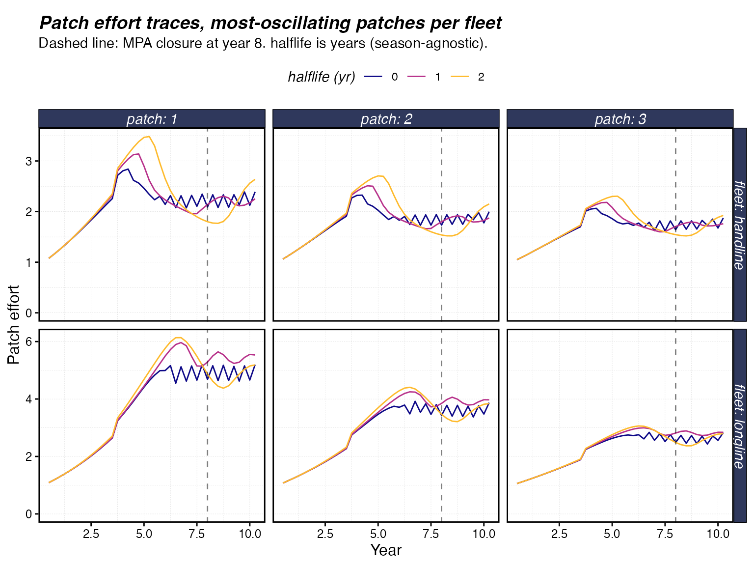
ggplot(trace_df, aes(year, effort, color = halflife)) +
  geom_line() +
  geom_vline(xintercept = mpa_year_5, linetype = "dashed", alpha = 0.5) +
  facet_grid(fleet ~ patch, scales = "free_y", labeller = label_both) +
  scale_y_continuous(limits = c(0,NA)) +
  scale_color_viridis_d(option = "C", end = 0.85) +
  labs(
    title    = "Patch effort traces, most-oscillating patches per fleet",
    subtitle = sprintf("Dashed line: MPA closure at year %d. halflife is years (season-agnostic).",
                       mpa_year_5),
    x = "Year", y = "Patch effort", color = "halflife (yr)"
  )

catch_ts <- purrr::map_dfr(runs_5, function(r) {
  r$proc$fauna %>%
    group_by(step) %>%
    summarise(catch = sum(c, na.rm = TRUE), .groups = "drop") %>%
    mutate(year = step * time_step,
           halflife = factor(r$halflife, levels = sort(unique(halflives_5))))
})

ggplot(catch_ts, aes(year, catch, color = halflife)) +
  geom_line() +
  geom_vline(xintercept = mpa_year_5, linetype = "dashed", alpha = 0.5) +
  scale_color_viridis_d(option = "C", end = 0.85) +
  labs(title = "Total catch over time",
       x = "Year", y = "Total catch", color = "halflife (yr)")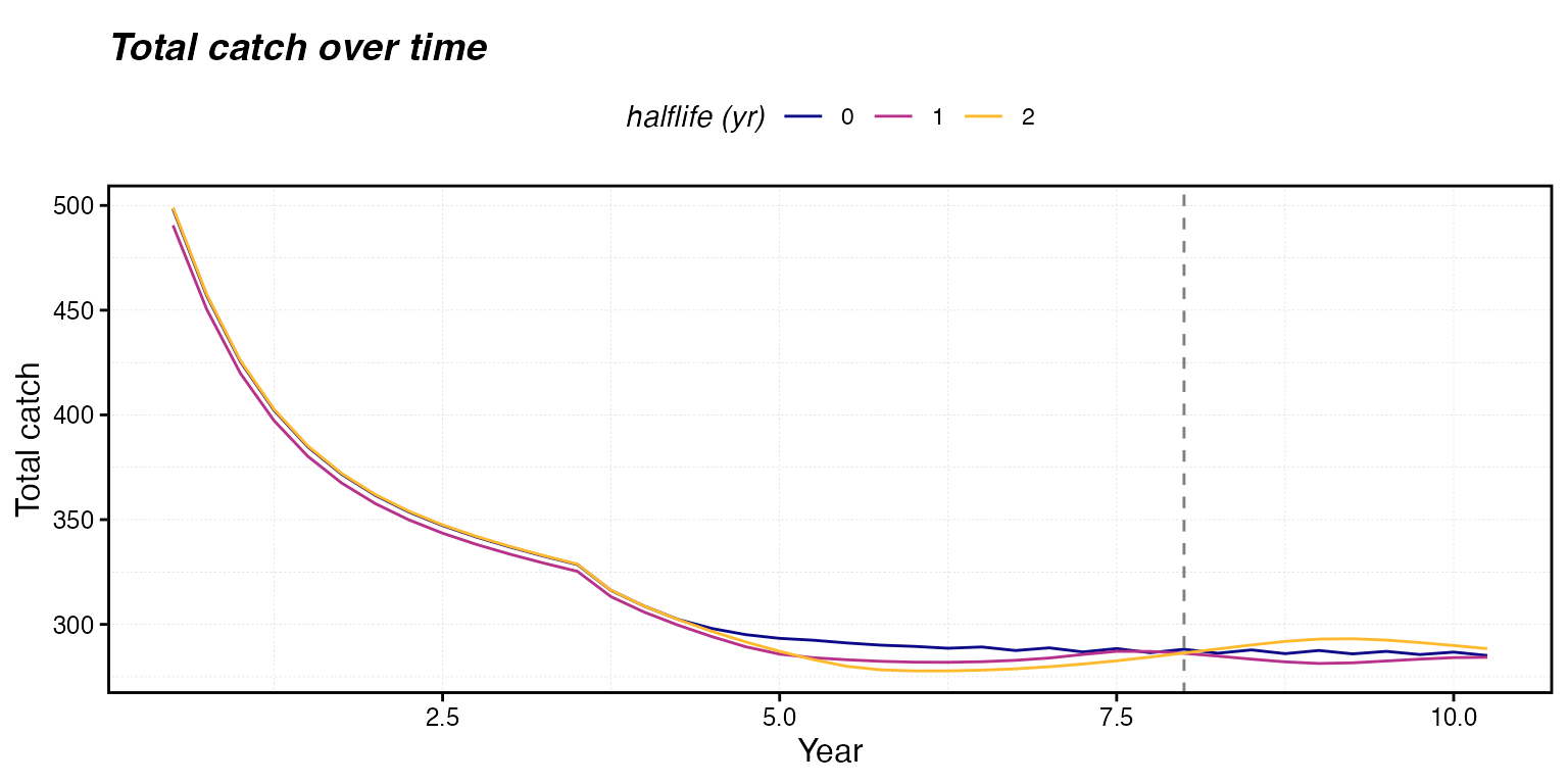

Reading the patch traces: halflife = 0 shows the high-frequency wiggle that motivates the parameter, sharpened further by the MPA closure. halflife = 1 (one year of memory) sits near the median of the sawtooth and removes the high-frequency component. halflife = 2 smooths further but begins to introduce slower swings driven by phase lag: the fleet’s perceived objective is now lagging the real one by ~3 years, so it reallocates toward patches that used to be high-value.

When does memory matter?

The susceptibility to one-step-lag oscillation depends strongly on a fleet’s configuration. Memory is not a universal upgrade; in many configurations it adds nothing or hurts.

Allocation strategy. marginal_profit and marginal_revenue have the most direct fleet-biomass feedback — the objective at a patch responds immediately to last step’s fishing there — and are the most prone to sawtooth. ppue / profit / rpue / revenue integrate over the production curve, which damps the feedback. manual and uniform ignore the buffet entirely, so memory does nothing for them (and is correctly skipped by simmar()).
Fleet model. constant_effort fleets have only the spatial-allocation feedback loop, so the spatial smoothing in memory is the only mechanism stabilising them. open_access and sole_owner fleets also adjust total effort each step from a fleet-wide profitability signal, which has its own slow damping built in via the annual entry/exit caps — but that signal itself is not smoothed by memory_halflife. If you observe sawtooth in total fleet effort (rather than in patch-level allocation), memory will not fix it; the right knob lives in the open-access / sole-owner parameters.
System structure. Strong fleet-biomass coupling (high catchability relative to stock productivity, fast movement that smooths biomass and equalises marginals, MPA closures that force redistribution) all amplify the one-step-lag feedback. Without any of these, the canonical scenarios in the main spatial-allocation vignette behave smoothly even at halflife = 0.

Sensible values for memory_halflife depend on the time scale of stock and fleet dynamics. For most marine fisheries with annual or sub-annual seasons, 0.5–1.5 years is a useful starting range. If catch or effort trajectories at a chosen halflife show slow swings that aren’t present at memory_halflife = 0, reduce it; you’ve crossed into the phase-lag regime. If the system is well-behaved at memory_halflife = 0, leave it there.